[DataCamp] Machine Learning with caret in R
This article is a summary of the eponymous course on DataCamp by Zachary Deane-Mayer ( LinkedIn) and Max Kuhn ( LinkedIn).
I learn by example and like to write code by starting from a previously-working template. The goal of this article is to have a reproducible example for later personal reference (and to make note of some personal corrections/updates). Readers are encouraged to take the interactive DataCamp course!
Template R code available in a GitHub Gist.
Article Contents
-
Regression models
Fit regression models withtrain()and evaluate out-of-sample performance using cross-validation and root mean square error (RMSE) -
Classification models
Fit classification models withtrain()and evaluate their out-of-sample performance using cross-validation and area under the curve (AUC) -
Random forests
Fit random forests and learn how to tune parameters via grid search -
Preprocessing
Usetrain()to preprocess data before fitting models, improving ability to make accurate predictions
Regression Models
In predictive (rather than explanatory) modeling, we want models that don't overfit the model and generalize well. Our primary concern is do the models perform well on new data?
We use metrics to evaluate the predictive accuracy of regression models.
Root Mean Square Error (RMSE)
Definition RMSE is a measure of model accuracy, defined as \[ RMSE = \sqrt{\frac{1}{n} \sum_{i=1}^n e_i^2} = \sqrt{\frac{1}{n} \sum_{i=1}^n (\hat y_i - y_i)^2} \] It is the average prediction error, looking at the difference between the prediction and the actual value. It is...
- the quantity minimized in linear regression
- one of the most common predictive error metrics
- an estimate of average error on the same scale as the outcome; says predictions are off by {rmse} units on average
In-sample RMSE is RMSE calculated with the same data used to estimate model parameters. This measure of RMSE can be too optimistic and lead to overfitting. It is better to calculate an out-of-sample estimate (based on predictions from data not used in model-fitting).
Cross-Validation
Definition Cross-validation (CV) is a method of evaluating out-of-sample error while reporting results fit on the full dataset.
It allows for the creation of multiple training/test sets, where each data point appears in a training set exactly once. Once you have calculated it, you refit your model on the entire dataset. The procedure is straight-forward:
- Divide the data into \(k\) (e.g., 10) folds.
- Use each fold as a test dataset and the remaining \(k-1\) as training.
- The smaller the dataset, the fewer folds.
- The split should approach 50/50 for smaller datasets (to create a more reliable test set).
- Check for overfitting by comparing the \(k\) different estimates of error
- If they are similar, we can feel more confident about the model's accuracy and the absence of overfitting.
- If they are different, the model does not perform consistently and this suggests a problem.
A cross-validated model is one where out-of-sample predictive error was evaluated using the steps above and identified as 'ok'.
To do cross-validation in R -- as well as diagnostic procedures like tuning and preprocessing like imputation -- we can use the caret package. The train() function allows for hundreds of different types of predictive models through the method argument. The repeats argument repeats the entire CV procedure (e.g., 5 times), thus yielding 50 error estimates.
Note that we pass the method for modeling to the main train() function and the method for cross-validation to trainControl().
-
trainControl()is also used for specification of custom modeling parameters -
if
trainControl()is defined externally, we can reuse it in multiple calls totrain() -
trainControl()contains a particular set of CV folds; it can be useful to define it externally and reuse the diff modeling procedures being considered
Classification Models
To fit a logistic regression model and generate predictions, we use
model1 <- glm(outcome ~ . , family = 'binomial' , ds)
p <- predict(model, new_ds, type = 'response')
Confusion Matrix
Definition A confusion matrix is a matrix of the model's predicted classes versus the true classifications. It's a tool used for evaluating the accuracy of binary classification models.
- Called such because it reveals how 'confused' the model is between the two classes, and highlights instances where one class is confused for the other.
-
The columns are the true classes while the rows are the predicted classes. The cell count true/false positives/negatives.
- The main diagonal of the confusion matrix are the cases where the model is correct.
- The second diagonal of the confusion matrix are the cases where the model is incorrect.
- The accuracy is the % correct classifications out of the total number (calculated on the test set).
- The no information rate is the % correct classifications out of the total number, when the model predicts everything as positive (calculated on the test set). A model is helpful when the accuracy is higher than this quantity.
- The sensitivity is the true positive rate, % true positives correctly identified as such (calculated on the test set).
- The specificity is the true negative rate, the % true negatives correctly identified as such (calculated on the test set).
To create a confusion matrix, we fit a logistic regression model and calculate the predicted probabilities. We then use those predictions to make a binary decision via defined threshold. We can use caret::confusionMatrix(predicted_class, true_class).
Calculation of a confusion matrix depends on what is used as the classification threshold.
-
Choosing a threshold is an exercise in balancing the true positive rate with the false positive rate.
-
Lower cutoff captures more positives, with less certainty about whether they are truly positives.
Used when we want to make sure we capture everything (e.g., there's a high consequence for missing something). -
Higher cutoff captures fewer positives, but with more certainty about whether they are truly positives.
Used when we want to feel confident about what we do identify (e.g., misclassification is expensive).
-
Lower cutoff captures more positives, with less certainty about whether they are truly positives.
- Choosing a threshold is somewhat dependent on a cost-benefit analysis of the problem at hand. Unfortunately there's not a good heuristic for choosing a cutoff ahead of time, you usually have to use a confusion matrix on your test set to find a good threshold.
Manually evaluating classification thresholds is hard. In order to do it correctly, we'd have to manually calculate dozens (or hundreds!) of confusion matrices, and then visually inspect them until we find one we like.
- Seems unscientific - requires lots of manual work, is heuristic-based, and could easily overlook an important threshold.
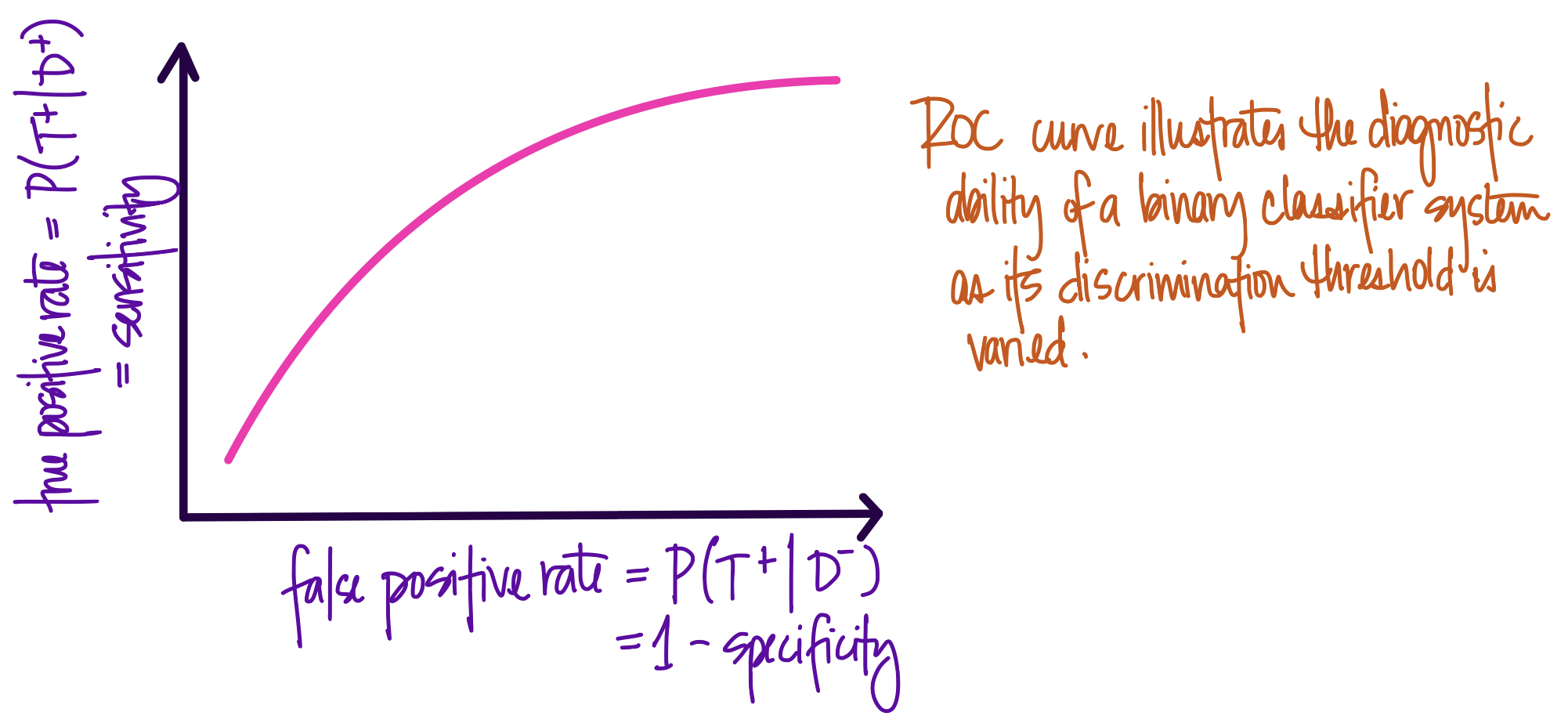
Definition A more systematic approach is to let a computer iteratively evaluate possible classification thresholds then calculate the true positive rate and false positive rate. We can then plot each true/false positive rate at every possible threshold and visualize the tradeoff between the two extremes - 100% true positive rate (i.e., predict everything as positive) versus 0% false positive (i.e., predict everything as negative). The resulting curve is called a receiver operating characteristic (ROC) curve.
- Developed during WWII as a method for analyzing radar signals. In this case, a true positive was correctly identifying a bomber by its radar signal, and a false positive is identifying a flock of birds as a bomber.
- The purpose of an ROC curve is to summarize the performance of a classifier over all possible thresholds.
- The \(x\)-axis is the false positive rate, and the \(y\)-axis is the true positive rate. Each point on the curve is a possible cutoff. Each point is a confusion matrix we don't have to calculate by hand.
When predicting classes randomly, the ROC curve will fall on the diagonal. On the other hand, models with a classification threshold that allows for perfect separation of classes will produce a 'box' with a single point at \((0,1)\) to represent a model where it is possible to achieve a 100% true positive rate and a 0% false positive rate.
Click to enlarge.
If we calculate the area under the ROC curves described above, we see that
- the area under the curve for a perfect model is exactly 1, since the plot represents a \(1 \times 1\) square
- the area under the curve for a random model is 0.5, since the plot represents a diagonal line
Definition We can use this insight to formalize a measure of model accuracy known as area under the curve (AUC).
- is a single-number summary of accuracy for logistic regression models
- calculated based on the ROC curve plot
- summarizes the model's performances across all possible classification thresholds
-
ranges from 0 to 1 where
- 0.0 is the AUC of a perfectly anti-predictive model (i.e., model is always wrong) (rare)
- 0.5 is the AUC of a random model (i.e., random guessing)
- 1.0 is the AUC of a perfect model (i.e., model is always right)
- in practice a model's AUC falls \( \in [0.5, 1.0] \) while a really bad model can occasionally be in the 0.4 range
- a rough rule of thumb is to think of AUC as a letter-grade
Random Forests
Random forests are a very popular type of machine learning model.
-
Advantages
- they're robust against overfitting
- require little preprocessing
- automatically capture threshold effects and interactions by default
- yield very accurate, nonlinear models with no extra work on the part of the data scientist
-
Disadvantages
- unlike linear models, they have hyperparameters to tune
-
unlike regular parameters (like the coefficients in a linear regression model, or the split points in a regression tree), the hyperparameters cannot be directly estimated from the training data
- they must be manually specified by the data scientist as inputs to the predictive model (i.e., before fitting the model)
- these hyperparameters control how the model fits to the data, and the optimal values for these parameters vary from dataset to dataset
- default values are often fine, but occasionally they aren't and will need adjustment
- can be slow
-
a 'black box' relative to
glmnet()
Random forests start with a simple decision tree model, which is fast but usually not very accurate. Random forests improve the accuracy of a single tree (i.e., model) via bootstrap aggregation (bagging): by fitting many trees, where each is fit to a different bootstrap sample of the original dataset. Random forests take bagging one step further by randomly re-sampling the columns of the dataset at each split. This additional level of sampling often yields even more accurate models. The package ranger (a reimplementation of randomForest) is great for fitting random forests in R and is often much faster + uses less memory than the original implementation.
- random forest : a tree is fit to a bootstrap sample; prediction is some average of the bootstrap predictions (similar to bagging)
- bagging : fitting trees to bootstrap samples (covariates for split randomly selected) then averaging; bootstrap aggregation
- boosting : summing many low-depth trees into a larger tree
Tuning
One of the big differences between a random forest and linear regression model is that random forests require tuning - heuristic discovery/specification of the hyperparameters.
An example of a hyperparameter that needs tuning is the number of randomly-selected variables used at each split in the individual decision trees that make up the random forest.
This is the only tuning parameter for random forests, mtry in ranger, an integer \(\in [2,100]\).
- Forests that use a covariate subset of size 2 tend to be more random, 100 variables tend to be less random.
- Hard to know the best value in advance, without trying them on the training data.
-
The function
caret::train()automates a process called grid search for selecting hyperparameters based on out-of-sample error, using the argumenttuneLength.- This argument is used to tell
train()to explore more models along its default tuning grid, wheretuneLength=10is a very fine tuning grid (default is3). This means we get a potentially more accurate model, but at the expense of waiting much longer for it to run.
- This argument is used to tell
-
We can then use
plot()to visually inspect the model's accuracy for different values ofmtry.- We select the
mtryvalue associated with the highest accuracy.
- We select the
-
To facilitate custom tuning, we can pass custom tuning grids via the
tuneGridargument incaret::train().- A tuning grid is created by creating a data frame with the values of the tuning parameters we want to explore.
-
If
tuneGridis not specified,train()will choose parameters automatically. - [pro] Most flexible method of fitting and tuning caret models.
- [pro] Gives full control over the models that are explored during grid search.
- [con] Requires advanced knowledge of how the model works.
- [con] A large/fine tuning grid can dramatically increase the model's runtime.
library(caret)
library(mlbench); data(Sonar)

# fitting a random forest using ranger pkg, caret pkg for cross validation
model <- train(Class ~.,
                data = Sonar,
                method = 'ranger', # pkg for fitting random forests
                tuneLength = 10,  # size of covar subset to use in fitting rdm forest
                tuneGrid = data.frame( .mtry = c(2, 3, 7),
                                       .splitrule = "variance",
                                       .min.node.size = 5 ), # specifying the tuning grid
                                                              # expand.grid() is cute too
                trControl = trainControl( method = "cv",
                                            number = 5,
                                            verboseIter = TRUE ))
model
plot(model)Lasso & Ridge Regression
glmnet models are an extension of generalized linear models (i.e., glm() in R) but have built-in variable selection.
- Helps linear regression models better handle collinearity (correlation among the predictors in a model).
- Prevents linear regression models from being over-confident in results derived from small sample sizes.
Definition There are two primary forms of glmnet models:
- Lasso regression which penalizes the number of non-zero coefficients
- Ridge regression which penalizes the absolute magnitude of the coefficients
Penalities are calculated during the model fit, and are used by the optimizer to adjust the linear regression coefficients. In other words, a glmnet attempts to find a parsimonious (simple) model, with either few non-zero coefficients, or small absolute magnitude coefficients, that best fit the input dataset. These are useful properties and pair well with random forest models.
glmnet models are a combination of lasso regression and ridge regression.
- They can fit a mix of lasso and ridge models (i.e., a model with a small penalty on both the number of non-zero coefficients and their absolute magnitude).
-
Thus glmnet models have many parameters to tune.
-
alpharanges from 0 to 1, where 0 is pure ridge and 1 is pure lasso regression; any value between is a mix of the two (i.e., an elastic net model) -
lambdaranges from 0 to \(+\infty\) and controls the size of the penalty; higher values of lambda will yield simpler models (1 is considered a large value, 10 is very large)- high enough values of lambda will yield intercept-only models that just predict the mean of the response variable in the training data
-
Random forest models are relatively easy to tune as there's really only one parameter of interest, mtry.
glmnet models have two parameters, alpha and lambda.
-
Trick! For a single value of
alpha, glmnet fits all values oflambdasimultaneously. - This is called the submodel trick because we can fit a number of different models simultaneously, and then explore the results of each submodel after the fact.
- We can also exploit this trick to get faster-running grid searches while still exploring finely-grained tuning grids.
-
When using glmnet as a method in
caret::train(),train()automatically chooses the correct parameters.
Preprocessing
Real world data have missing values. This is a problem for most statistical or machine learning algorithms: they usually require numbers to work with, and don't know what to do with missing data.
- The complete case approach is common, where the analyst throws out rows with missing data, but this is generally not a good idea. It can lead to biases in your dataset and generate over-confident models. In extreme cases, you'll end up throwing out all your data.
- A better strategy is median imputation, using the median to guess what a missing value would be, if it weren't missing. This is a very good idea if your data are missing at random and lets you include rows with missing values in the modeling.
Median imputation can be specified via the preProcess = 'medianImpute' argument to caret::train(). MI is fast but can produce incorrect results if the data are MNAR. (Tree-based models tend to be robust to the MNAR case.)
One useful type of missing value imputation is k-nearest neighbors (KNN) imputation.
- This is a strategy for imputing missing values based on other 'similar' non-missing rows.
- It tries to overcome the MNAR problem by inferring what the missing values would be based on observations that are similar in other, non-missing variables.
-
Can be specified via the
preProcess = 'knnImpute'argument totrain().
The preProcess argument to caret::train() can do a lot more than missing value imputation.
-
One can also chain together multiple preprocessing steps.
For example, a common recipe for preprocessing data prior to fitting a linear model is- median imputation
- center data
- scale data
- fit a glm
-
Preprocessing 'cheat sheet'
- start with median imputation
- try KNN imputation if MNAR
- for linear models, always center and scale
- for linear models, try PCA and spatial sign because this can sometimes yield better results
- tree-based models such as random-forests or GBMs typically don't need much preprocessing
library(caret)

# Apply median imputation: median_model
median_model <- train(
    x = breast_cancer_x,
    y = breast_cancer_y,
    method = 'glm',             # logistic regression
    trControl = myControl,
    preProcess = c('medianImpute', 'center', 'scale')   # or can be just one preprocessing step
                                                        # see ?preProcess for more info
)

# Print median_model to console
median_model
Comparing Models
When comparing models, make sure they're fit on the same data / CV folds!
-
Do this by using the same
trainControl()across models -
Use
resamples()to summarize different models' performance across folds (numerically and graphically)
model_list = list(glmnet = train_output1,
                  rf = train_output2)
summary(resamples(model_list))Handling Low-Information Predictors
In the real world, the data we're using for predictive modeling is often messy. Some variables in our dataset might not contain much information.
- Variables that are constant (zero variance) or close to constant (low variance) don't contain much useful information and it can sometimes be useful to remove them prior to modeling.
- Low variance predictors can sometimes yield constant columns within a CV fold. Constant columns can mess up a lot of models and should be avoided.
-
[TIP] Remove extremely low variance predictors from dataset prior to modeling. They have little information and thus tend not to have an impact on the results of the model. We can also reduce model-fitting time this way.
-
The utility function
nearZeroVar()can be used to remove the constant covariates. It usesfreqCut\( = \frac{\text{most common value}}{\text{second most common value}} \) anduniqueCut\( = \frac{\text{\# distinct values}}{\text{sample size}} \).
Recommended values are 2 and 20 respectively. -
The arguments
zvandnzvdo the same thing asnearZeroVar().
-
The utility function
# MANUALLY REMOVE LOW VAR COVARIATES
# Identify near zero variance predictors: remove_cols
remove_cols <- nearZeroVar(bloodbrain_x, names = TRUE,
                           freqCut = 2, uniqueCut = 20)

# Get all column names from bloodbrain_x: all_cols
all_cols = names(bloodbrain_x)

# Remove from data: bloodbrain_x_small
bloodbrain_x_small <- bloodbrain_x[ , setdiff(all_cols, remove_cols)]Principle Component Analysis
Principle Component Analysis (PCA) is another potential preprocessing step for linear regression models.
- Combines low variance and correlated variables in the dataset into a single set of high variance, perpendicular predictors.
- Better to find to find a systematic way to use those low variance and/or correlated variables, rather than throw them away - is an alternative to junking low variance predictors.
- Perpendicular covariates are useful because they're perfectly uncorrelated; thus PCA can remove issues of collinearity.
- PCA searches for high-variance linear combinations of the input data, that are perpendicular to each other. The first component of PCA is the highest-variance component, and is the highest variance axis of the original data. The second component has the second-highest variance... and so on.
-
pcacan be specified as an argument topreProcess: this will center and scale the data, combine low variance variables, and ensure that all predictors are orthogonal.
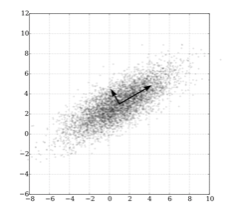
The diagram at left shows how PCA works. We have two correlated variables, \(x\) and \(y\). PCA transforms the data with respect to this correlation, and finds a new variable (the long arrow) that reflects the shared correlation of \(x\) and \(y\). This first component reflects the similarity between \(x\) and \(y\). After finding the first PCA component, the second is constrained to be perpendicular; it reflects the difference between \(x\) and \(y\).