[DataCamp] Introduction to Natural Language Processing in R
This article is a summary of the eponymous course on DataCamp by Kasey Jones ( LinkedIn).
I learn by example and like to write code by starting from a previously-working template. The goal of this article is to have a reproducible example for later personal reference (and to make note of some personal corrections/updates). Readers are encouraged to take the interactive DataCamp course!
Template R code available in a GitHub Gist.
Article Contents
Analysis Methods
True Fundamentals
Natural language processing (NLP) focuses on using computers to analyze and understand text.
Regular expressions
Regular expressions are sequences (bka patterns) used to search text.
My favorite website to validate regular expressions is RegEx 101.
| Pattern | What's matched in the text |
R example | Match example |
|---|---|---|---|
| \w | any single alphanumeric character | gregexpr(pattern = '\\w', text) | a |
| \d | any single digit | gregexpr(pattern = '\\d', text) | 1 |
| \w+ | any alphanumeric string, any length | gregexpr(pattern = '\\w+', text) | word |
| \d+ | consecutive digits, any length | gregexpr(pattern = '\\d+', text) | 1234 |
| \s | a single space | gregexpr(pattern = '\\s', text) | ' ' |
| \S | a single character that's not a space | gregexpr(pattern = '\\S', text) | w |
| ? |
0 or 1 of whatever character follows it (not to be used alone) |
gregexpr(pattern = '(?i)boxer', text) | Boxer or boxer |
| i | case insensitivity |
gregexpr(pattern = '(?i)boxer', text) (?i) is an example of negative lookahead and this pattern enables case insensitivity for the remainder of the expression. |
Boxer or boxer |
There are a number of functions in R for using regular expressions.
| Function | Purpose | Syntax |
|---|---|---|
|
grep()
(base R) |
find matches of the pattern in a vector |
grep(pattern = '\w', x = strVec, value = FALSE)
note value = TRUE prints the text instead of the indices; FALSE is the default. |
|
gsub()
(base R) |
replaces all matches of the regular expression in a string or vector | gsub(pattern = '\d+', replacement = "", x = strVec) |
Tokenization
Definition Tokenization is the act of splitting text into individual tokens. To tokenize text is to split it into tokens.
Definition A token is a meaningful unit of text, most often a word, that we are interested in using for further analysis, and tokenization is the process of splitting text into tokens ( definition source).
Tokens can be as small as individual characters, or as large as the entire text document. Common types of tokens are characters, words, sentences, and documents. We could even separate text into custom units based on a regular expression (e.g., splitting text every time I see a 3+ digit number).
One common R package for text mining is tidytext. The function for tokenization is unnest_tokens(). It takes data frame tbl and extracts tokens from the column input. We also specify what kind of tokens we want with the argument token and what the output column should be labeled with the argument output.
The example below demonstrates how to use tidytext::unnest_tokens(), as well as using count() to count token frequency. animal_farm is a dataframe with two columns, chapter and text_column. There are 10 rows, one for each chapter in the book. The result of unnest_tokens() is a data frame with two columns, chapter and word. There are 30,037 rows in this particular result, one for each token in animal_farm.
library(dplyr)
library(tidytext)

# convert to a tibble, easier to print
animal_farm <- read.csv('animal_farm.csv',
                        stringsAsFactors = FALSE) %>%
               as_tibble()
animal_farm
# A tibble: 10 x 2
chapter text_column
<chr> <chr>
1 Chapter 1 "Mr. Jones, of the Manor Farm, had locked the hen-…
2 Chapter 2 "Three nights later old Major died peacefully in h…
3 Chapter 3 "How they toiled and sweated to get the hay in! Bu…
4 Chapter 4 "By the late summer the news of what had happened …
5 Chapter 5 "As winter drew on, Mollie became more and more tr…
6 Chapter 6 "All that year the animals worked like slaves. But…
7 Chapter 7 "It was a bitter winter. The stormy weather was fo…
8 Chapter 8 "A few days later, when the terror caused by the e…
9 Chapter 9 "Boxer's split hoof was a long time in healing. Th…
10 Chapter 10 "Years passed. The seasons came and went, the shor…
animal_farm %>%
    unnest_tokens(output = 'word',
                  input  = text_column,
                  token  = 'words') %>%
    # sort by most frequent token to least
    count(word, sort = TRUE) %>%
    head()
      word    n
    1  the 2187
    2  and  966
    3   of  899
    4   to  814
    5  was  633
    6    a  620
Another use of unnest_tokens() is to find all mentions of a particular word and see what follows it. In Animal Farm, Boxer is one of the main characters. We can check what Chaper 1 says about him.
animal_farm %>%
    filter(chapter == 'Chapter 1') %>%
    unnest_tokens(output = 'Boxer',
                  input  = text_column,
                  token  = 'regex',
                  pattern = '(?i)boxer') %>%
    # select all rows except the first one
    slice(2:n())
  # A tibble: 5 x 2
    chapter   Boxer
    <chr>      <chr>
  1 Chapter 1 " and clover, came in together, walking very slowly …
  2 Chapter 1 " was an enormous beast, nearly eighteen hands high,…
  3 Chapter 1 "; the two of them usually spent their sundays toget…
  4 Chapter 1 " and clover; there she purred contentedly throughou…
  5 Chapter 1 ", the very day that those great muscles of yours lo…
Here we have filtered Animal Farm to Chapter 1, and looked for any mention of Boxer, regardless of capitalization. Since the first token starts at the beginning of the text, we're using slice() to skip the first token. The output is the text that follows every mention of Boxer.
Text cleaning basics
To demonstrate some techniques, we'll use a portion of the Russian troll tweets dataset by FiveThirtyEight. First let's tokenize by words then calculate frequencies.
library(dplyr)
library(tidytext)

# convert to a tibble, easier to print
russian_tweets <- read.csv('russian_1.csv',
                           stringsAsFactors = FALSE) %>%
                  as_tibble()
russian_tweets
# A tibble: 20,000 x 22
X external_author… author content region language
<int> <dbl> <chr> <chr> <chr> <chr>
1 1 9.06e17 10_GOP "\"We … Unkno… English
2 2 9.06e17 10_GOP "Marsh… Unkno… English
3 3 9.06e17 10_GOP "Daugh… Unkno… English
4 4 9.06e17 10_GOP "JUST … Unkno… English
5 5 9.06e17 10_GOP "19,00… Unkno… English
6 6 9.06e17 10_GOP "Dan B… Unkno… English
7 7 9.06e17 10_GOP "🐝🐝🐝 h… Unkno… English
8 8 9.06e17 10_GOP "'@Sen… Unkno… English
9 9 9.06e17 10_GOP "As mu… Unkno… English
10 10 9.06e17 10_GOP "After… Unkno… English
# … with 19,990 more rows, and 16 more variables:
# publish_date <chr>, harvested_date <chr>, following <int>,
# followers <int>, updates <int>, post_type <chr>,
# account_type <chr>, retweet <int>, account_category <chr>,
# new_june_2018 <int>, alt_external_id <dbl>, tweet_id <dbl>,
# article_url <chr>, tco1_step1 <chr>, tco2_step1 <chr>,
# tco3_step1 <chr>
russian_tweets %>%
    unnest_tokens(word, content) %>%
    count(word, sort = TRUE)
  # A tibble: 44,318 x 2
    word      n
    <chr> <int>
  1 t.co  18121
  2 https 16003
  3 the    7226
  4 to     5279
  5 a      3623
  6 in     3422
  7 of     3211
  8 is     2951
  9 and    2720
 10 you    2465
 # … with 44,308 more rows
Definition The most frequent words are not helpful and we should remove them before analysis. Such words are referred to as stop words and are typically the most common words in a language (e.g., the, and in English). To remove these stop words from our text before analysis, we can perform an tidytext::anti_join() function using the stop_words tibble provided by tidytext.
stop_words
  # A tibble: 1,149 x 2
    word        lexicon
    <chr> <int>
  1 a           SMART
  2 a's         SMART
  3 able        SMART
  4 about       SMART
  5 above       SMART
  # … with 1,144 more rows
tidy_tweets <- russian_tweets %>%
    # tokenize the 'content' column in russian_tweets
    # save the results in a column named 'word'
    unnest_tokens(output = word,
                  input  = content) %>%
    anti_join(stop_words)

tidy_tweets %>% count(word, sort = TRUE)
  # A tibble: 43,666 x 2
     word                n
    <chr>            <int>
  1 t.co             18121
  2 https            16003
  3 http              2135
  4 blacklivesmatter  1292
  5 trump             1004
  # … with 43,661 more rows
We can add our own stop words https, http, and t.co to stop_words.
custom <- add_row(stop_words, word = "https", lexicon = "custom")
custom <- add_row(custom, word = "http", lexicon = "custom")
custom <- add_row(custom, word = "t.co", lexicon = "custom")
russian_tweets %>%
    unnest_tokens(output = word,
                  input  = content) %>%
    anti_join(custom) %>%
    count(word, sort = TRUE)
  # A tibble: 43,663 x 2
   word                 n
   <chr>            <int>
 1 blacklivesmatter  1292
 2 trump             1004
 3 black              781
 4 enlist             764
 5 police             745
# … with 43,658 more rows
Definition Another text cleaning technique is stemming, the process of transforming words into their roots. For example, both enlisted and enlisting would be trimmed to their root enlist. Stemming is an important step when trying to understand which words are being used.
To transform our tokens into their roots we can use SnowballC::wordStem().
library(SnowballC)
tidy_tweets <- russian_tweets %>%
    unnest_tokens(output = word,
                  input  = content) %>%
    anti_join(custom)
# stemming
stemmed_tweets <- tidy_tweets %>%
    mutate(word = wordStem(word))

stemmed_tweets %>% count(word, sort = TRUE)
  # A tibble: 38,907 x 2
    word               n
    <chr>          <int>
  1 blacklivesmatt  1301
  2 cop             1016
  3 trump           1013
  4 black            848
  5 enlist           809
  6 polic            763
  7 peopl            730
  8 rt               653
  9 amp              635
 10 policebrut       614
 # … with 38,897 more rows
Representations of Text
Definition A corpus (plural corpora) is a collection of text. Corpora are collections of documents containing natural language text. A common representation of this in R is the Corpus class from the tm package. A VCorpus (volatile corpus) is used to host both the text and metadata. To demonstrate use of VCorpus, we'll use the acq dataset from tm. It contains a subset of articles (50) from the Reuters dataset.
library(tm)
data("acq")
To access the first article in acq, we can use list index notation. Metadata for a particular article can be accessed via meta.
# meta data, first article
acq[[1]]$meta
    author       : character(0)
    datetimestamp: 1987-02-26 15:18:06
    description  :
    heading      : COMPUTER TERMINAL SYSTEMS  COMPLETES SALE
    id           : 10
    language     : en
    origin       : Reuters-21578 XML
    topics       : YES
    lewissplit   : TRAIN
    cgisplit     : TRAINING-SET
    oldid        : 5553
    places       : usa
    people       : character(0)
    orgs         : character(0)
    exchanges    : character(0)
Furthermore, we can access individual objects within meta.
names(acq[[1]]$meta)
 [1] "author"        "datetimestamp" "description"   "heading"
 [5] "id"            "language"      "origin"        "topics"
 [9] "lewissplit"    "cgisplit"      "oldid"         "places"
[13] "people"        "orgs"          "exchanges"
acq[[1]]$meta$places
[1] "usa"
A VCorpus contains the text of each document within content. Below is the truncated text of the first article.
acq[[1]]$content
[1] "Computer Terminal Systems Inc said\nit has completed the sale
of 200,000 shares of its common\nstock, and warrants to acquire
an additional one mln shares, to\n<Sedio N.V.> of Lugano,
Switzerland for 50,000 dlrs.\n    The company said the warrants
are exercisable for five\nyears at a purchase price of .125
dlrs per share....
To do analysis on these data using functions from the tidytext package, we'll need to prepare a tidier version. In order to get the data into a table format, where each observation is represented by a row and each variable by a column, we can use tidy() function on a VCorpus. This function extracts the metadata and content and saves it in a tibble.
tidy_data <- tidy(acq)
tidy_data
# A tibble: 50 x 16
    author datetimestamp       description heading id
    <chr>  <dttm>              <chr>       <chr>   <chr>
  1 <NA>   1987-02-26 09:18:06 ""          COMPUT… 10
  2 <NA>   1987-02-26 09:19:15 ""          OHIO M… 12
  3 <NA>   1987-02-26 09:49:56 ""          MCLEAN… 44
  4 By Ca… 1987-02-26 09:51:17 ""          CHEMLA… 45
  5 <NA>   1987-02-26 10:08:33 ""          <COFAB… 68
  6 <NA>   1987-02-26 10:32:37 ""          INVEST… 96
  7 By Pa… 1987-02-26 10:43:13 ""          AMERIC… 110
  8 <NA>   1987-02-26 10:59:25 ""          HONG K… 125
  9 <NA>   1987-02-26 11:01:28 ""          LIEBER… 128
 10 <NA>   1987-02-26 11:08:27 ""          GULF A… 134
 # … with 40 more rows, and 11 more variables:
 #   language <chr>, origin <chr>, topics <chr>,
 #   lewissplit <chr>, cgisplit <chr>, oldid <chr>,
 #   places <named list>, people <lgl>, orgs <lgl>,
 #   exchanges <lgl>, text <chr>
Conversely, if we want to do analysis on these data using functions from tm, we can convert a tibble to a VCorpus using VCorpus() and VectorSource(). Combined, these functions create a VCorpuscorpus from the text content. To add metadata, use meta() to add columns to the metadata dataframe attached to the corpus.
corpus <- VCorpus(VectorSource(tidy_data$text))
meta(corpus, 'Author') <- tidy_data$author
meta(corpus, 'oldid') <- tidy_data$oldid
head(meta(corpus))
                     Author oldid
1                      <NA>  5553
2                      <NA>  5555
3                      <NA>  5587
4 By Cal Mankowski, Reuters  5588
5                      <NA>  5611
6                      <NA>  5639
The bag-of-words representation
Consider the following three strings.
text1 <- c('Few words are important.')
text2 <- c('All words are important.')
text3 <- c('Most words are important.')
The bag-of-words representation uses vectors to specify which words are in each string: we find the unique words, and then convert this information into vector representations.
-
few - only in
text1 -
all - only in
text2 -
most - only in
text3 - words, are, and important is present in all strings
Definition The first step is to create a clean vector of the unique words used in all of the text to be analyzed. Although this is project-dependent, to clean text usually means
- using lower-cased words
- no stop words
- no punctuation
- converting to stemmed words
# lowercase, without stop words
word_vector <- c('few', 'all', 'most', 'words', 'important')
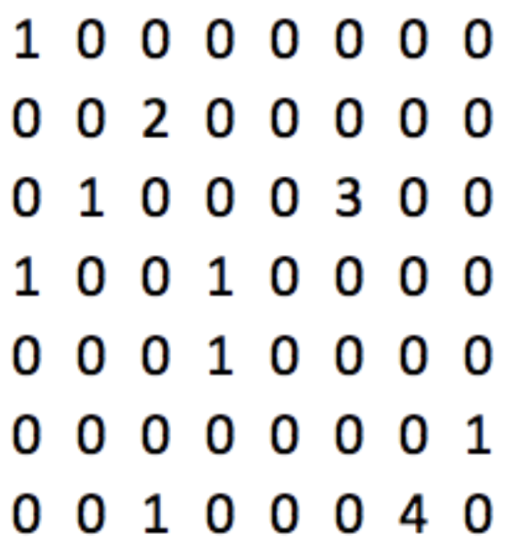
We then convert each string into a binary representation of which words are in that text. Although below is a binary representation, we could have used word counts.
# representation for text1
text1 <- c('Few words are important.')
text1_vector <- c(1,0,0,1,1)

# representation for text2
text2 <- c('All words are important.')
text2_vector <- c(0,1,0,1,1)

# representation for text3
text3 <- c('Most words are important.')
text3_vector <- c(0,0,1,1,1)
The tidytext package uses a representation that more manageable for larger text. To find the words that appear in each chapter of animal_farm, we can use the familiar process of unnest_tokens(), anti_join(), and count(). The result is a tibble of word counts by chapter, sorted from most to least common.
words <- animal_farm %>%
    unnest_tokens(output = 'word',
                  token  = 'words',
                  input  = text_column) %>%
    anti_join(stop_words) %>%
    # count column 'chapter' and group by 'word'
    count(chapter, word, sort = TRUE)
# word frequency count, by chapter
words
 # A tibble: 6,807 x 3
   chapter    word         n
  <chr>      <chr>    <int>
 1 Chapter 8  napoleon    43
 2 Chapter 8  animals     41
 3 Chapter 9  boxer       34
 4 Chapter 10 animals     32
 5 Chapter 10 farm        30
 6 Chapter 5  animals     28
 7 Chapter 7  snowball    28
 8 Chapter 7  animals     27
 9 Chapter 9  animals     27
10 Chapter 2  animals     26
# … with 6,797 more rows
In the binary vector representation, a document that does not contain a word receives a 0 for that word. In this representation, chapter and word pairs that do not exist are left out. The key difference is that in the former, the absence of a word is explicitly stated.
Napoleon, interestingly enough, is a main character but is not mentioned in chapter 1.
words %>%
    filter(word == 'napoleon') %>%
    arrange(desc(n))
# A tibble: 9 x 3
  chapter    word         n
  <chr>      <chr>    <chr>
1 Chapter 8  napoleon    43
2 Chapter 7  napoleon    24
3 Chapter 5  napoleon    22
4 Chapter 6  napoleon    15
5 Chapter 9  napoleon    13
6 Chapter 10 napoleon    11
7 Chapter 2  napoleon     9
8 Chapter 3  napoleon     3
9 Chapter 4  napoleon     1
From the Russian troll tweets dataset by FiveThirtyEight, we're using a subset of 20,000 tweets out of over 3 million original tweets. The subset contains over 43,000 unique, non-stop words.
tidy_tweets <- russian_tweets %>%
    unnest_tokens(word, content) %>%
    anti_join(stop_words)
tidy_tweets %>% count(word, sort = TRUE)
 # A tibble: 43,666 x 2
   word                 n
   <chr>            <int>
 1 t.co             18121
 2 https            16003
 3 http              2135
 4 blacklivesmatter  1292
 5 trump             1004
 6 black              781
 7 enlist             764
 8 police             745
 9 people             723
10 cops               693
# … with 43,656 more rows
Credit: DataCamp video.
Tweets are short, with most tweets only containing a handful of words. With these 20,000 tweets and 43,000 words we create a sparse matrix. Each row is a tweet and each column a word, a 20,000 x 43,000 matrix. In our case, we would need 860 million values, but only 177,000 would be non-zero, about 0.02%!
Representing text as vectors can use a lot of computational resources, and most would be spent on storing zeros. As we see from the example above, there would be very few non-zero entries. R packages like tidytext and tm help relieve this burden by storing the values in a smart and efficient manner.
Term frequency-inverse document frequency matrix (TFIDF)
Consider these three pieces of text.
t1 <- 'My name is John. My best friend is Joe. We like tacos.'
t2 <- 'Two common best friend names are John and Joe.'
t3 <- 'Tacos are my favorite food. I eat them with my friend Joe.'
After cleaning this text, we get the following.
clean_t1 <- 'john friend joe tacos'
clean_t2 <- 'common friend john joe names'
clean_t3 <- 'tacos favorite food eat buddy joe'
When comparing (clean) t1 and t2, they share almost every single word - 3/4 of words from t1 are in t2. 3/5 words from t2 are in t1. However when comparing t1 and t3, they don't seem to share that many words. 2/4 words from t1 are in t3. 2/6 words from t3 are in t1. So t1 and t2 must be more similar than t1 and t3!
Let's return to the original text. One word that matters above all others is tacos. All three texts have John and Joe, but only two texts share John, Joe, and tacos. This is the main idea behind why we use the term frequency-inverse document frequency matrix.
Definition The TFIDF is a way of representing word counts by considering two components.
-
the term frequency (TF), the proportion of words in a text that are that specific term.
example TF(John,clean_t1) = 1/4 -
the inverse document frequency, which considers how frequent words appear relative to the full collection of text.
example John appears in all three (cleaned) texts, so IDF(John) = 1 - 3/3 = 0.The IDF actually has several different calculation methods. The most common form is \[ IDF = \ln\left( \frac{N}{n_t} \right) \] where
- \(N\) is the total number of documents in the corpus
- \(n_t\) is the number of documents where the term appears
We can quickly calculate the IDF for other words.
- IDF(taco) = \(\ln(\frac{3}{2}) = 0.405\)
- IDF(buddy) = \( \ln(\frac{3}{1}) = 1.10 \)
- IDF(John) = \( \ln(\frac{3}{3}) = 0 \)
The TFIDF is the product of the TF and IDF, whose calculation relies on the above bag-of-words representation. It's a measure of how 'relevant' a token is in the corpus ( details), but is calculated for each document-word. If a token (e.g., word) shows up frequently in a document, the TF will be high; but if that word shows up frequently in all documents (e.g., the word the) then the IDF will balance out the TF. The TFIDF allows us to compare token importance across documents. TFIDF is zero when it appears in all the documents, or it doesn't appear in a particular document. As an example, the TFIDF value for tacos associated with each text is calculated below.
-
clean_t1: TF × IDF = \( \frac{1}{4} \times 0.405 = 0.101 \) -
clean_t2: TF × IDF = \( \frac{0}{4} \times 0.405 = 0 \) -
clean_t3: TF × IDF = \( \frac{1}{6} \times 0.405 = 0.068 \)
The tidytext function bind_tf_idf() can be used to calculate the TFIDF for each token in a corpus.
df <- data.frame('text' = c(t1, t2, t3),
                 'ID' = c(1,2,3),
                 stringsAsFactors = FALSE)
df %>%
    unnest_tokens(output = 'word',
                  token = 'words',
                  input = text) %>%
    anti_join(stop_words) %>%
    # count column 'ID' and group by 'word'
    count(ID, word, sort = TRUE) %>%
    # 'term' is the column w the terms
    # 'document' is the column w the doc/string ID
    # 'n' is the column w the doc-string counts
    bind_tf_idf(term = word, document = ID, n)
       ID     word n        tf       idf     tf_idf
    1   1   friend 1 0.2500000 0.0000000 0.00000000
    2   1      joe 1 0.2500000 0.0000000 0.00000000
    3   1     john 1 0.2500000 0.4054651 0.10136628
    4   1    tacos 1 0.2500000 0.4054651 0.10136628
    5   2   common 1 0.2000000 1.0986123 0.21972246
    6   2   friend 1 0.2000000 0.0000000 0.00000000
    7   2      joe 1 0.2000000 0.0000000 0.00000000
    8   2     john 1 0.2000000 0.4054651 0.08109302
    9   2    names 1 0.2000000 1.0986123 0.21972246
    10  3      eat 1 0.1666667 1.0986123 0.18310205
    11  3 favorite 1 0.1666667 1.0986123 0.18310205
    12  3     food 1 0.1666667 1.0986123 0.18310205
    13  3   friend 1 0.1666667 0.0000000 0.00000000
    14  3      joe 1 0.1666667 0.0000000 0.00000000
    15  3    tacos 1 0.1666667 0.4054651 0.06757752
Cosine similarity
Cosine similarity is a measure of similarity between two non-zero vectors. Applied here, it's used to assess how similar two articles are. The value 0 means the two articles are perpendicular, i.e., they share no non-common words. The value 1 means the articles are identical. Use cases are situations when we need to assess similarity between texts.
We can calculate the cosine similarity between every pair of articles using pairwise_similarity() from the widyr package. The example below compares the chapters of Animal Farm.
animal_farm %>%
      unnest_tokens(word, text_column) %>%
      # create word counts
      count(chapter, word) %>%
      # calculate cosine similarity by chapter,
      # using words and their counts
      # 'item' = documents to compare (articles, tweets, etc)
      # 'feature' = link between docs (i.e., words)
      # 'value' = numeric value for each feature
      #           (e.g., counts or tfidf)
      pairwise_similarity(item = chapter, word, n) %>%
      arrange(desc(similarity))
  # A tibble: 90 x 3
    item1      item2      similarity
    <chr>      <chr>           <dbl>
  1 Chapter 9  Chapter 8       0.972
  2 Chapter 8  Chapter 9       0.972
  3 Chapter 8  Chapter 7       0.970
  4 Chapter 7  Chapter 8       0.970
  5 Chapter 8  Chapter 10      0.969
  6 Chapter 10 Chapter 8       0.969
  7 Chapter 9  Chapter 5       0.968
  8 Chapter 5  Chapter 9       0.968
  9 Chapter 9  Chapter 10      0.966
 10 Chapter 10 Chapter 9       0.966
 # … with 80 more rows
Classification and Topic Modeling
Preparing text for modeling
In this example we'll use classification modeling to classify sentences by the character being discussed, Napoleon or Boxer. To prepare the text, we'll
- tokenize the corpus into sentences
- label the sentences based on whether napoleon or boxer was used
- replace mentions of napoleon or boxer (so classification algorithm doesn't use it when training)
- limit sentences under consideration to those that mention Boxer or Napoleon, but not both
# tokenize into sentences
sentences <- animal_farm %>%
    unnest_tokens(output = "sentence",
                  token  = "sentences",
                  input  = text_column)

# label sentences by animal
# grepl() returns TRUE when the pattern is found in
#   the indicated string
sentences$boxer <- grepl('boxer', sentences$sentence)
sentences$napoleon <- grepl('napoleon', sentences$sentence)

# replace animal names
sentences$sentence <- gsub("boxer", "animal X", sentences$sentence)
sentences$sentence <- gsub("napoleon", "animal X", sentences$sentence)

# limit sentences to those with exactly one mention
#   of either napoleon or boxer (not both)
animal_sentences <- sentences[sentences$boxer + sentences$napoleon == 1,]

# add label to new cleaned dataset
animal_sentences$name <- as.factor(ifelse(animal_sentences$boxer,
                                          "boxer",
                                          "napoleon"))

# select a subset as our final dataset
animal_sentences <- rbind(animal_sentences[animal_sentences$name == "boxer",][c(1:75),],
                          animal_sentences[animal_sentences$name == "napoleon",][c(1:75),])
animal_sentences$sentence_id <- 1:nrow(animal_sentences)
animal_sentences
  # A tibble: 150 x 6
    chapter  sentence        boxer napoleon name  sentence_id
    <chr>    <chr>           <lgl> <lgl>    <fct>       <int>
  1 Chapter… the two cart-h… TRUE  FALSE    boxer           1
  2 Chapter… animal X was a… TRUE  FALSE    boxer           2
  3 Chapter… nevertheless, … TRUE  FALSE    boxer           3
  4 Chapter… last of all ca… TRUE  FALSE    boxer           4
  5 Chapter… you, animal X,… TRUE  FALSE    boxer           5
  6 Chapter… animal X was f… TRUE  FALSE    boxer           6
  7 Chapter… only old benja… TRUE  FALSE    boxer           7
  8 Chapter… the animals ha… TRUE  FALSE    boxer           8
  9 Chapter… when animal X … TRUE  FALSE    boxer           9
 10 Chapter… some hams hang… TRUE  FALSE    boxer          10
 # … with 140 more rows
For classification models, we create a document-term matrix (DTM) with TFIDF weights using the cast_dtm() function from tidytext. A DTM is a matrix with one row per document (sentence in this case) and one column for each word.
animal_matrix <- animal_sentences %>%
    unnest_tokens(output = 'word',
                  token  = 'words',
                  input  = sentence) %>%
    anti_join(stop_words) %>%
    mutate(word = wordStem(word)) %>%
    # count words by sentence
    count(sentence_id, word) %>%
    cast_dtm(document  = sentence_id,
             term      = word,
             value     = n,
             weighting = tm::weightTfIdf)
animal_matrix
<<DocumentTermMatrix (documents: 150, terms: 694)>>
    Non-/sparse entries: 1221/102879
    Sparsity           : 99%
    Maximal term length: 17
    Weighting          : term frequency - inverse document frequency (normalized) (tf-idf)
In this example, we have 150 sentences and 694 unique words. However, most words are not in each sentence: the output tells us that 1,221 of the 150 * 694 = 104,100 entries in this DTM are populated and 102,879 entries are equal to zero. The sparsity is 102,879/104,100 = 99%.
Using large, sparse matrices makes the computational part of modeling difficult, taking a lot of time and/or memory. We can improve computation resource usage by removing sparse terms (i.e., tokens, here words) from the analysis using removeSparseTerms() from tm.
- The sparse argument specifies the maximum sparseness we'll tolerate.
- The sparse argument can be determined through trial-and-error, by trying different levels and checking how many terms are left.
- In the examples below, removing sparse terms brings the number of terms down from 694 to 3 and 172, respectively.
- It's computationally trivial to do analysis with the full matrix, so we'll move forward without removing any terms.
removeSparseTerms(animal_matrix, sparse = 0.90)
<<DocumentTermMatrix (documents: 150, terms: 3)>>
    Non-/sparse entries: 181/269
    Sparsity           : 60%
    Maximal term length: 7
    Weighting          : term frequency - inverse document frequency (normalized) (tf-idf)
removeSparseTerms(animal_matrix, sparse = 0.99)
<<DocumentTermMatrix (documents: 150, terms: 172)>>
    Non-/sparse entries: 699/25101
    Sparsity           : 97%
    Maximal term length: 10
    Weighting          : term frequency - inverse document frequency (normalized) (tf-idf)
Classification modeling
First let's separate our dataset into training and test sets.
set.seed(1111)
sample_size <- floor(0.80 * nrow(animal_matrix))
train_ind   <- sample(nrow(animal_matrix), size = sample_size)
train <- animal_matrix[train_ind, ]
test  <- animal_matrix[-train_ind, ]
Next we fit a random forest model to do our classification.
- The unit of analysis is a sentence.
-
The covariates are the 694 unique words, but provided as vectors of indicators reflecting whether that word was used in a particular sentence. These vectors were created by
cast_dtm. - The outcome is whether a particular sentence discussed napoleon or boxer.
library(randomForest)
rfc <- randomForest(x = as.data.frame(as.matrix(train)),
                    y = animal_sentences$name[train_ind],
                    nTree = 50)
rfc
Call:
    randomForest(x = as.data.frame(as.matrix(train)),
                 y = animal_sentences$name[train_ind],
                 nTree = 50)

                  Type of random forest: classification
                        Number of trees: 500
   No. of variables tried at each split: 26

           OOB estimate of  error rate: 25.83%
   Confusion matrix:
            boxer napoleon class.error
   boxer       46       13    0.220339
   napoleon    18       43    0.295082
The confusion matrix for the training dataset suggests an accuracy of 74%.
-
Rows of the matrix represent the actual labels, columns represent the predicted labels.
- Out of 46 + 13 = 59 sentences whose true class was boxer, 13 were classified incorrectly by the model.
- Out of 18 + 43 = 61 sentences whose true class was napoleon, 18 were classified incorrectly by the model.
- The overall accuracy of the model on the training set is the fraction of total sentences that was labelled correctly: (46 + 43) / (46 + 13 + 18 + 43) = 0.74
We use predict() to generate predictions on the test dataset and table() to calculate the confusion matrix.
y_pred <- predict(rfc, newdata = as.data.frame(as.matrix(test)))
# generate confusion matrix
table(animal_sentences[-train_ind,]$name, y_pred)
          y_pred
         boxer napoleon
boxer       15        1
napoleon     7        7
-
Rows of the matrix represent the actual labels, columns represent the predicted labels.
- Out of 15 + 1 = 16 sentences whose true class was boxer, 1 was classified incorrectly by the model.
- Out of 7 + 7 = 14 sentences whose true class was napoleon, 7 were classified incorrectly by the model.
- The overall accuracy of the model on the training set is the fraction of total sentences that was labelled correctly: (15 + 7) / (15 + 1 + 7 + 7) = 0.73
Topic modeling
A collection of text is likely to be made up of a collection of topics. One of the most common algorithms for topic modeling is latent Dirichlet allocation ( LDA), which uses two basic principles:
- Each document is made up of a small mixture of topics.
- The presence of a word in each document can be attributed to a topic.
In order to perform LDA, we need a DTM with term frequency weights. We give this matrix to LDA() from the topicmodels package, where parameter k is the number of topics.
animal_farm_matrix <- animal_farm %>%
    unnest_tokens(output = "word",
                  token  = "words",
                  input  = text_column) %>%
    anti_join(stop_words) %>%
    mutate(word = wordStem(word)) %>%
    # cast word counts into a DTM
    count(chapter, word) %>%
    cast_dtm(document = chapter,
             term = word,
             value = n,
             weighting = tm::weightTf)

library(topicmodels)
animal_farm_lda <- LDA(train,
                       k = 4,   # number of topics
                       method = 'Gibbs',
                       control = list(seed = 1111))
animal_farm_lda
A LDA_Gibbs topic model with 4 topics
Next we use tidy() to extract terms and their corresponding \(\beta\) coefficient for each topic. Generally speaking, \(\beta\) is a per-topic word distribution. It explains how related to each topic a term is. Words more related to a single topic will have a higher \(beta\) value.
animal_farm_betas <- tidy(animal_farm_lda, matrix = "beta")
  # A tibble: 11,004 x 3
    topic term beta
    <int>   <chr>     <dbl>
 5      1 abolish 0.0000360
 6      2 abolish 0.00129
 7      3 abolish 0.000355
 8      4 abolish 0.0000381
...
Also note that the sum of these \(\beta\)s should be equal to the total number of topics.
sum(animal_farm_betas$beta)
[1] 4
Characterizing Topics Let's look at the top words per topic. For topic 1 we see words like napoleon, animal, and windmill.
# characterizing topics with their assoc words
animal_farm_betas %>%
    group_by(topic) %>%
    top_n(10, beta) %>%
    arrange(topic, -beta) %>%
    filter(topic == 1)
    topic     term      beta
    <int>    <chr>     <dbl>
 1      1 napoleon    0.0339
 2      1     anim    0.0317
 3      1  windmil    0.0144
 4      1 squealer    0.0119
...
For topic 2, we see similar words to topic 1. This might indicate that we need to remove some of the non-entity words such as animal and rerun our analysis.
# characterizing topics with their assoc words
animal_farm_betas %>%
    group_by(topic) %>%
    top_n(10, beta) %>%
    arrange(topic, -beta) %>%
    filter(topic == 2)
    topic     term      beta
    <int>    <chr>     <dbl>
...
 3      2 anim        0.0189
...
 6      2 napoleon    0.0148
...
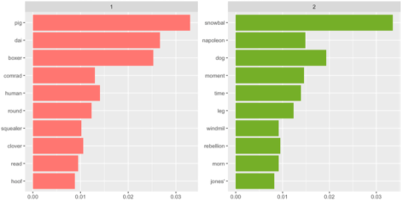
Click to enlarge.
Credit: tidytext manual via a DataCamp video
The figure on the right is a visualization of results from rerunning LDA after removing animal and farm. It's not a good idea to remove too many words, but since the book is called Animal Farm, it made sense to do so. Topic 1 appears to be more about pig, daisy, and boxer, while topic 2 is focused on snowball and napoleon and dogs.
Assigning Topics to Documents The words of each chapter are used to assign topics to them. To extract the topic assignments, we can use tidy() but specify that we need the gamma matrix. The gamma matrix represents how much of the chapter is made up of a single topic.
Chapter 1 is mostly comprised of topic 3, with a little of topics 1 and 2 as well.
animal_farm_chapters <- tidy(animal_farm_lda,
                             matrix = "gamma")
animal_farm_chapters %>%
    filter(document == "Chapter 1")
  # A tibble: 4 x 3
    document    topic    gamma
    <chr>       <int>    <dbl>
1   Chapter 1       1    0.157
2   Chapter 1       2    0.136
3   Chapter 1       3    0.623
4   Chapter 1       4    0.0838
LDA in practice
LDA will create the topics for you, but it won't tell you how many to create. The perplexity metric a measure of how well a probability model fits new data.
- lower value is better
- used to compare models in LDA parameter tuning and/or selecting the number of topics
To use perplexity in model development:
- create a train/test split of the data - we must assess perplexity on the testing dataset to make sure our topics are also extendable to new data
-
create LDA models - for each k we train a model and calculate the perplexity score using
topicmodels::perplexity() - plot the perplexity values with k on the \(x\)-axis
# create train/test split
sample_size <- floor(0.90 * nrow(doc_term_matrix))
set.seed(1111)
train_ind <- sample(nrow(doc_term_matrix), size = sample_size)
train <- matrix[ train_ind,]
test  <- matrix[-train_ind,]

# create LDA models
values <- c()
for(j in 2:35) {
    lda_model <- LDA(train, k = j, method = "Gibbs",
                     control = list(iter = 25, seed = 1111))
    values <- c(values, perplexity(lda_model, newdata = test))
}

# plot perplexity values
plot(c(2:35), values, main = "Perplexity for Topics",
     xlab = "Number of Topics", ylab = "Perplexity")
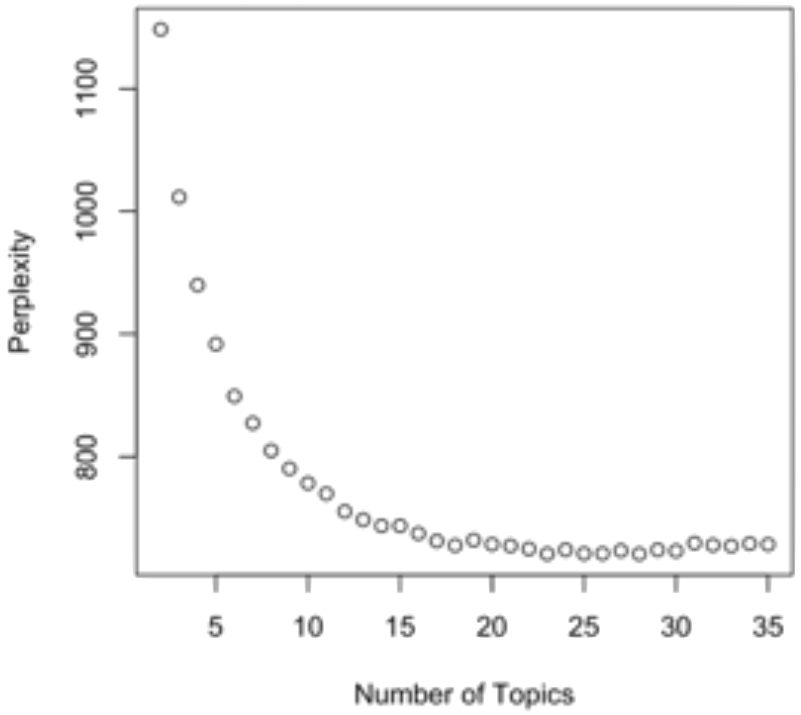
Click to enlarge.
Credit: DataCamp video
In the plot on the left, notice that between 12 and 15 topics, the perplexity score doesn't improve much with the addition of more topics. We gain no real value by using more than 15 topics. Based on the plot, we should use a model with 10 to 15 topics.
LDA is more often about practical use than it is about selecting the optimal number of topics based on perplexity.
- A collection of articles might comprise 15-20 topics, but describing 20 topics to an audience might not be feasible.
- Visuals with only 4-5 topics are a lot easier to comprehend than graphics with 100 topics.
-
[Rule of thumb] Use a small number of topics where each topic is represented by a large number of documents.
- If there's time, >10 topics can be used for exploration and dissection
- It's common to have a subject matter expert review the top words in a topic to provide a theme, then confirm with the top documents in the topic. Repeat for each topic.
Summarizing Output Count how many times each topic was the highest-weighted topic for a particular document. In the example output below, topic 1 was the top topic for 1,326 documents.
gammas <- tidy(lda_model, matrix = "gamma")
gammas %>%
    group_by(document) %>%
    arrange(desc(gamma)) %>%
    slice(1) %>%
    group_by(topic) %>%
    tally(topic, sort = TRUE)
      topic      n
 1        1   1326
 2        5   1215
 3        4    804
...
Summarizing Output View how strong a topic was when it was the top topic. Topic 1 had the highest average weight when it was the top topic.
gammas %>%
    group_by(document) %>%
    arrange(desc(gamma)) %>%
    slice(1) %>%
    group_by(topic) %>%
    summarize(avg = mean(gamma)) %>%
    arrange(desc(avg))
      topic     avg
 1        1   0.696
 2        5   0.530
 3        4   0.482
...
Advanced Techniques
Sentiment analysis
Sentiment analysis is used to assess the subjective information in text, e.g.,
- positive versus negative
- words elicit some form of emotion
To perform sentiment analysis, we start with a dictionary of words that have a predefined value or score, e.g.,
- abandon might be related to fear
- accomplish might be related to joy
In tidytext there are three dictionaries (bka lexicons) for us to use. Each have advantages when used in the right context; before an analysis we must decide what type of sentiment we want to extract from the text available.
As discussed in Tidy Text Mining with R, all three lexicons are based on unigrams (single words). The function get_sentiments() allows us to get specific lexicons with the appropriate measures for each one.
Lexicons are enumerated below with descriptions from Tidy Text Mining with R. Details on how these lexicons were curated are located there. Note that each have license requirements that should be reviewed before use.
The AFINN lexicon assigns words with a score that runs between -5 (extremely negative) and 5 (extremely positive). Negative scores indicate negative sentiment and positive scores indicate positive sentiment.
library(tidytext)
library(textdata)
get_sentiments("afinn")
 # A tibble: 2,477 x 2
   word       value
   <chr>       <chr>
 1 abandon       -2
 2 abandoned     -2
 3 abandons      -2
 4 abducted      -2
 5 abduction     -2
 6 abductions    -2
 7 abhor         -3
 8 abhorred      -3
 9 abhorrent     -3
10 abhors        -3
# … with 2,467 more rows
The bing lexicon categorizes words in a binary manner into positive and negative categories.
get_sentiments("bing")
  # A tibble: 6,786 x 2
    word        sentiment
    <chr>       <chr>
  1 2-faces     negative
  2 abnormal    negative
  3 abolish     negative
  4 abominable  negative
  5 abominably  negative
  6 abominate   negative
  7 abomination negative
  8 abort       negative
  9 aborted     negative
 10 aborts      negative
 # … with 6,776 more rows
The nrc lexicon categorizes words in a binary fashion (yes/no) into categories of positive, negative, anger, anticipation, disgust, fear, joy, sadness, surprise, and trust.
get_sentiments("nrc")
  # A tibble: 13,901 x 2
    word        sentiment
    <chr>       <chr>
  1 abacus      trust
  2 abandon     fear
  3 abandon     negative
  4 abandon     sadness
  5 abandoned   anger
  6 abandoned   fear
  7 abandoned   negative
  8 abandoned   sadness
  9 abandonment anger
 10 abandonment fear
 # … with 13,891 more rows
To use these lexicons for sentiment analysis, our data needs to be tokenized. Note how, for sentiment analysis we did not perform stemming as words might create different feelings than just their stem.
# read in the data
animal_farm <- read.csv("animal_farm.csv",
                        stringsAsFactors = FALSE) %>%
               as.tibble()

# tokenize and remove stop words
animal_farm_tokens <- animal_farm %>%
                      unnest_tokens(output = "word",
                                    token  = "words",
                                    input  = text_column) %>%
                      anti_join(stop_words)
Once we have the tokens, we can join the words with their sentiment by using an inner join. The results are a new tibble with each word and its sentiment. Since the AFINN lexicon uses scores from -5 to 5, we see the scores as its own column.
animal_farm_tokens %>%
    inner_join(get_sentiments("afinn"))
 # A tibble: 1,175 x 3
    chapter   word        value
    <chr>     <chr>       <dbl>
  1 Chapter 1 drunk          -2
  2 Chapter 1 strange        -1
  3 Chapter 1 dream           1
  4 Chapter 1 agreed          1
  5 Chapter 1 safely          1
  6 Chapter 1 stout           2
  7 Chapter 1 cut            -1
  8 Chapter 1 comfortable     2
  9 Chapter 1 care            2
 10 Chapter 1 stout           2
 # … with 1,165 more rows
We can take this a step further, by grouping the sentiments by chapter and summarizing the overall score. The results make sense! For example, Chapter 7 is about a cold winter during which the animals struggle to rebuild their farm.
animal_farm_tokens %>%
    inner_join(get_sentiments("afinn")) %>%
    group_by(chapter) %>%
    summarise(sentiment = sum(value)) %>%
    arrange(sentiment)
  # A tibble: 10 x 2
    chapter    sentiment
    <chr>          <dbl>
  1 Chapter 7       -166
  2 Chapter 8       -158
  3 Chapter 4        -84
  4 Chapter 9        -56
  5 Chapter 10       -49
  6 Chapter 2        -45
  7 Chapter 6        -44
  8 Chapter 1        -15
  9 Chapter 5        -15
 10 Chapter 3          7
The bing lexicon labels words as strictly positive or negative. Instead of summarizing the scores, we count the total words and the number of negative words - by document, in this case by chapter.
We find results similar to what we found with the AFINN lexicon. Chapter 7 contains the highest proportion of negative words used at almost 12%.
# total # words by chapter
word_totals <- animal_farm_tokens %>%
    group_by(chapter) %>%
    count()

# calc proportion negative words
animal_farm_tokens %>%
inner_join(get_sentiments("bing")) %>%
    group_by(chapter) %>%
    count(sentiment) %>%
    filter(sentiment == 'negative') %>%
    transform(p = n / word_totals$n) %>%
    arrange(desc(p))
          chapter sentiment   n          p
    1   Chapter 7  negative 154 0.11711027
    2   Chapter 6  negative 106 0.10750507
    3   Chapter 4  negative  68 0.10559006
    4  Chapter 10  negative 117 0.10372340
    5   Chapter 8  negative 155 0.10006456
    6   Chapter 9  negative 121 0.09152799
    7   Chapter 3  negative  65 0.08843537
    8   Chapter 1  negative  77 0.08603352
    9   Chapter 5  negative  93 0.08462238
    10  Chapter 2  negative  67 0.07395143
The nrc lexicon labels words as positive or negative, but also fear, anger, trust, and others. We can use this lexicon to see if certain emotions might be in our text.
as.data.frame(table(get_sentiments('nrc')$sentiment)) %>%
    arrange(desc(Freq))
               Var1 Freq
    1      negative 3324
    2      positive 2312
    3          fear 1476
    4         anger 1247
    5         trust 1231
    6       sadness 1191
    7       disgust 1058
    8  anticipation  839
    9           joy  689
    10     surprise  534
We know that Animal Farm is about animals overthrowing their human rulers; let's see what words related to fear are in the text. rebellion, death, and gun are the most common 'fear'-related words in the text.
fear <- get_sentiments('nrc') %>%
    filter(sentiment == 'fear')
animal_farm_tokens %>%
    # limit analysis to only words labeled as 'fear'
    inner_join(fear) %>%
    count(word, sort = TRUE)
  # A tibble: 220 x 2
    word           n
    <chr>      <int>
  1 rebellion     29
  2 death         19
  3 gun           19
  4 terrible      15
  5 bad           14
  6 enemy         12
  7 broke         11
  8 attack        10
  9 broken        10
 10 difficulty     9
 # … with 210 more rows
Word embeddings
Consider the two equivalent statements below, with and without stop words (stop words in gray). Because smartest and brilliant are not the same word, traditional similarity metrics would not do well here.
- Bob is the smartest person I know.
- Bob is the most brilliant person I know.
But what if we used a system that had access to hundreds of other mentions of smartest and brilliant? And instead of just counting how many times each word was used, we also had information on which words were used in conjunction with those words?
word2vec is one of the most popular word embedding methods around, developed in 2013 by a team at Google.
- Uses a large vector space to represent words.
- Built such that words of similar meaning are closer together.
- Built such that words appearing together often will be closer together in a given vector space.
The implementation of word2vec() being used here comes from the h2o package, one of many machine learning libraries in R.
- min_word_freq removes words used fewer than the specified number
- epochs number of training iterations to run (use a larger number for larger amounts of text)
- performs best if the model has enough data to properly train; if words are not mentioned enough in the dataset, the model might not be useful
library(h2o)

# start an h2o instance
h2o.init()

# convert tibble into an h2o object
h2o_object <- as.h2o(animal_farm)

# tokenize using h2o
words <- h2o.tokenize(h2o_object$text_column, "\\\\W+")
words <- h2o.tolower(words) (chapter)
# place NA after last word of each document
#  and remove stop words
words <- words[is.na(words) || (!words %in% stop_words$word),]

word2vec_model <- h2o.word2vec(words,
                               min_word_freq = 5,
                               epochs = 5)
There are several uses for this word2vec model, but we'll use it here to find similar terms. The function h2o.findSynonyms() helps us see that the word animal is most related to words like mind, agreed, announced.
h2o.findSynonyms(word2vec_model, "animal")
          synonym     score
    1        mind 0.9890062
    2      agreed 0.9878455
    3   announced 0.9870282
    4       crept 0.9868813
The name of the character Jones, who is the enemy of the animals in the book, is most related to words like difficult and enemies.
h2o.findSynonyms(word2vec_model, "jones")
          synonym     score
    1     enemies 0.9922917
    2  excitement 0.9918446
    3   difficult 0.9914268
    4    speeches 0.9914203
The book Animal Farm only has about 10,000 non-stop words. We'd likely see even better results with more text.
Additional NLP analysis tools
Bidirectional Encoder Representations from Transformers (BERT) was released by Google in 2017. It is a model that we can use with transfer learning to complete NLP tasks. It's pretrained, meaning that it has already created a language representation by training on a ton of unlabeled data. When we use BERT, it only takes a small amount of labeled data to train BERT for a specific supervised learning task. BERT is also great at creating features that can be used in NLP models.
Other knoweldge integration language representations like Enhanced Representation through kNowledge IntEgration (ERNIE) have recently come out and are improving NLP analysis.
Named entity recognition is not a new method, but it seeks to classify named entities within text. Examples of named entities are names, locations, organizations, and sometimes values, percentages, and even codes. Named entity recognition can be used for tasks such as
- extracting entities from tweets that mention a company name
- aiding recommendation engines by recommending similar content or products
- creating efficient search algorithms, as documents or text can be tagged with the entities that are found within them
Even older than named entity recognition is part-of-speech tagging. It is a simple process that involves tagging each word with the correct part-of-speech. each word is labeled as a noun, verb, adjective, or other type of speech. Part-of-speech tagging is used across the NLP landscape. It's used to aid in
-
sentiment analysis
(the more you know about a sentence, the better you can understand the sentiment) -
create features for NLP models
(can enhance what a model knows about the words being used)