Fundamentals of causal inference, part 1:
Assumptions + the assignment mechanism
Causal inference refers to an intellectual discipline that considers the assumptions, study designs, and estimation strategies that allow researchers to draw causal conclusions based on data.
Contents
- The Stable Value Treatment Assumption
- Strong Ignorability
- Estimating the Causal Effect
- The Assignment Mechanism
- Example 1
- Example 2
- Example 3
Causal inference is a collection of tools that allow us to make causal statements about an intervention and the subsequent outcome. There are great philosophical discussions on what constitutes a cause but this discussion will be statistical.
As stated by Imbens & Rubin, the problem of causal inference is a missing data problem: given any treatment assigned to an individual unit, the potential outcome associated with any alternate treatment is missing, or unobserved. Let the causal effect be defined as a comparison of potential outcomes. Because of the Fundamental Problem -- the fact that we can only observe one potential outcome -- estimation of the causal effect from data requires assumptions.
The Stable Value Treatment Assumption (SUTVA)
Definition The two components of SUTVA are:
- The potential outcomes for any unit do not vary with the treatments assigned to other units (i.e., no interference).
- There are no different forms or versions of each treatment level, which lead to different potential outcomes (i.e., treatments must be well-defined).
Strong Ignorability
Some notation
Let \(i\) index individuals within a finite sample of size \(n\), randomly sampled from a much larger population of interest. \(W_i \in \{0,1\}\) is a binary indicator of an individual's point exposure status and \(\mathbf{X}_i\) a \( p \)-dimensional vector of measured pre-treatment variables (aka covariates aka attributes). Lowercase \( w_i \), \(\mathbf{x}_i\) are realizations of their uppercase counterparts. \( Y_i(w_i) \) represents the potential outcomes that would have been observed had individual \(i\) been assigned to treatment or control.
Definition Ignorability is the independence of the potential outcomes and treatment, conditional on covariates \(\mathbf{X}\): \[ \left( Y_i(0), Y_i(1) \right) \perp\!\!\!\perp W_i \,\, | \,\, \mathbf{X}_i \quad \forall \; i \] This condition is often referred to as "no unmeasured confounding" or "unconfoundedness".
Strong ignorability is the version of ignorability assumed in this discussion, which involves the additional condition that it is possible to observe both treated and untreated units within every level of \(\mathbf{X}\): \[ \left( Y_i(0), Y_i(1) \right) \perp\!\!\!\perp W_i \,\, | \,\, \mathbf{X}_i \quad \text{ and } \quad \Pr(W_i = 1 \, | \, \mathbf{X}_i) \in (0,1) \quad \quad \forall \; i \]
Estimating the Causal Effect
On the difference scale, the causal effect of treatment on individual \(i\) is \( Y_i(1) - Y_i(0) \). The Fundamental Problem precludes observation of this individual treatment effect (ITE), so we instead consider the average treatment effect (ATE) as our estimand, defined as an average over the entire population. We're able to estimate the ATE from observed data under the assumptions of SUTVA and strong ignorability. Note that SUTVA and strong ignorability are recast as (conditional)
exchangeability,
consistency, and
positivity
in the epidemiological context. How these recharacterizations are used is described below.
(Unit subscripts \(i\) omitted for clarity.)
\[
\begin{aligned}
E\left[ Y(1) - Y(0) \, | \, \mathbf{X} \right] & = E\left[ Y(1) \, | \, \mathbf{X} \right] - E\left[ Y(0) \, | \, \mathbf{X} \right]
& \text{(1)}
\\
& = E\left[ Y(1) \, | \, W = 1, \mathbf{X}\right] - E\left[ Y(0) \, | \, W = 0, \mathbf{X} \right]
& \text{ (2)}
\\
& \phantom{=} \text{\color{blue}(by conditional exchangeability)}
\\
& = E[Y^{obs} | W = 1, \mathbf{X} = \mathbf{x}] - E[Y^{obs} | W = 0, \mathbf{X} = \mathbf{x}]
& \text{\color{blue}(by consistency)} \text{ (3)}
\\
E\left[ Y(1) - Y(0) \right] & = E_{F_{\mathbf{X}}}\left\{
E[Y^{obs} | W = 1, \mathbf{X} = \mathbf{x}] - E[Y^{obs} | W = 0, \mathbf{X} = \mathbf{x}]
\right\}
& \text{\color{blue} (ATE)} \text{ (4)}
\end{aligned}
\]
Note that the ATE defined in \((4)\) is one of several possible causal estimands.
Nevertheless, SUTVA and strong ignorability are the assumptions that allow us to equate the conditional expectations of potential outcomes to conditional expectations of observed outcomes.
Hernán & Robins
and
Morgan & Winship.
There are variables associated with both \(W\) and \(Y\) such that the quantity measured in \((4)\) is not a treatment effect, but a spurious measure of association that is in part due to dissimilarities in their distribution across treatment arms. These problematic covariates are referred to as confounders, defined here as the subset of \(\mathbf{X}\) required for strong ignorability to hold. For the purposes of this discussion, we assume that the covariates measured in \(\mathbf{X}\) contain (at least) all confounders required to satisfy the assumption of strong ignorability and estimate causal treatment effects.
The Assignment Mechanism
A key role is played by the missing data mechanism, or, as referred to in the causal inference context, the assignment mechanism. How is it determined which units get treatments? Equivalently, how is it determined which potential outcomes are realized and which are not? Answers to these questions help to determine the \(\mathbf{X}\) required for strong ignorability to hold and the appropriate analysis procedure for our data.
Definition The assignment mechanism is the process that determines which units receive which treatments, hence which potential outcomes are realized and which are missing. Formally, it is the assignment of probability to each of the possible treatment vectors (where a treatment vector is a vector of length \(n\), a possible assignment of treatment to each of the units in the sample of size \(n\)).
There are three basic restrictions on (or, properties of) assignment mechanisms.
- Individualistic
- An assignment mechanism is individualistic when each unit-level probability of treatment does not depend on the potential outcomes or covariates of other units.
- Probabilistic
- An assignment mechanism is probabilistic when each unit's treatment assignment probability is between 0 and 1, but not equal to 0 or 1.
- Unconfounded
- An assignment mechanism is unconfounded when it does not depend on the potential outcomes (but can depend on covariates).
There are several classes of assignment mechanisms, defined by which of the restrictions/properties are fulfilled.
- Randomized
-
A randomized experiment is an assignment mechanism that
- is probabilistic, and
- has a known functional form that is controlled by the researcher.
- Classical Randomized
-
A classical randomized experiment is a randomized experiment with an assignment mechanism that is
- individualistic, and
- unconfounded.
Other prominent examples of classical randomized experiments include stratified randomized experiments and paired randomized experiments. - Observational
- An assignment mechanism corresponds to an observational study if the functional form of the assignment mechanism is unknown.
- Regular
-
An assignment mechanism is regular if
- the assignment mechanism is individualistic,
- the assignment mechanism is probabilistic, and
- the assignment mechanism is unconfounded.
If, in addition, the functional form of regular assignment is not known, the assignment mechanism corresponds to an observational study with a regular assignment mechanism. - Irregular
-
An assignment mechanism is irregular if
assignment to treatment differs (for at least some units) from the receipt of treatment.
We assume that assignment to treatment itself is unconfounded, but allow receipt of treatment to be confounded.
This class of assignment mechanisms includes noncompliance in randomized experiments and sometimes utilizes instrumental variables analysis.
Example 1
Question from Ec1127 course offered at Harvard University and taught by Prof. Cassandra Pattanayak.
During a check-up, a physician find that his patient's thyroid levels are too low. He prescribes medication at a high dose and asks her to be retested in a month. At the second test, the patient's thyroid levels are now too high, so the physician switches her to a low dose of medication and again asks her to be retested in a month. At the third test, the patient's thyroid levels are perfect, so the doctor decides that she should stay at the low dose indefinitely.
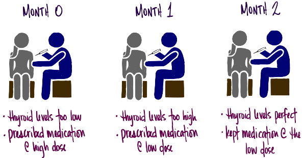
Question 1.1 What are the units?
- the patient after zero months
- the patient after one month
- the patient after two months
- ...(there could potentially be more months, depending on the thyroid level of the patient after two months and the doctor's subsequent diagnostic decision)
Question 1.2 What is the treatment?
- \( W_i = 0 : \) low dose
- \( W_i = 1 : \) high dose
Question 1.3 What are the potential outcomes?
- \( Y_1(0) \) is the thyroid level after the first month (second visit) under low dose.
- \( Y_1(1) \) is the thyroid level after the first month (second visit) under high dose.
- \( Y_2(0) \) is the thyroid level after the second month (third visit) under low dose.
- \( Y_2(1) \) is the thyroid level after the second month (third visit) under high dose.
| \( i \) | \( Y_i(0) \) | \( Y_i(1) \) |
|---|---|---|
| patient at month zero (\( i = 1\)) | unknown/unobserved | high thyroid level |
| patient at month one (\( i = 2\)) | perfect thyroid level | unknown/unobserved |
| patient after ... months (\( i = \ldots\)) |
Question 1.4 Is SUTVA possible?
Solution 1.4 Assessing theoretical plausibility is different from practical plausibility (e.g., including additional medical knowledge to assess plausibility). The statements below assess theoretical plausibility.
-
[Part 1] No interference: Plausible.
The requirement is that the treatment applied to one unit (thyroid medication to the patient at a particular point in time) does not affect the potential outcomes for other unit (patient at a different point in time). In other words, the effect of the medication doesn't last for more than a month. -
[Part 2] Well-defined treatments: Plausible.
The requirement is that the amount of the dose in low dose or high dose, or the administration of the dose, cannot alter the potential outcome for any unit. This is plausible.
Question 1.5 Why must SUTVA be plausible for us to conceptualize the Science table?
Solution 1.5 SUTVA allows us to properly enumerate all the potential outcomes associated with each unit. In other words, SUTVA allows us to clearly enumerate each row of the Science table. When we write \(Y_i(0)\) we are assuming that it is well-defined:
- its value doesn't depend on the treatment assignment of other units (SUTVA 1)
- unambiguous (SUTVA 2)
Question 1.6 Do you agree with the physician's judgement that the patient should remain on the low dose, given the information provided here?
Note that determination of a causal effect needs an appropriate reference potential outcome, e.g., \(Y(\text{no dose})\). In this case, the physician is likely comparing \( Y_3(\text{low dose}) \) with \( Y_3(\text{high dose}) \) and assuming \( Y_3(\text{low dose}) \) leads to a better health outcome.
Question 1.7 Does the physician's assignment mechanism appear probabilistic? Individualistic? Unconfounded?
Solution 1.7 The physician's assignment mechanism is the process s/he uses to determine how to treat the patient. Properties of the assignment mechanism are considered below.
- [Probabilistic] Maybe because we don't know whether the probability of treatment is bounded away from zero; we don't know enough about how the doctor assigned treatment.
- [Individualistic] No because the assignment mechanism for Unit 3 (i.e., the process that determines what treatment the patient receives at month two) depends on the treatment & potential outcomes for Unit 2 (the patient at month one).
- [Unconfounded] No because the assignment mechanism (i.e., the process that determines what treatment the patient receives) depends on the potential outcomes... the physician prescribes based on what s/he thinks the potential outcomes are.
Example 2
Question from Ec1127 course offered at Harvard University and taught by Prof. Cassandra Pattanayak.
Suppose that the federal Department of Education surveys school districts to find out how many male and female teachers are employed in each district. The Department learns that some school districts have been hiring only female teachers. Rather than intervene directly in hiring, the Department creates a workshop for school administrators that focuses on the benefits of diversity. The workshop is given at all school districts that currently have only female teachers. At other school districts across the country, the workshop is given if requested by school administrators. Two years later, the Department again asks all school districts to indicate the number of male and female teachers employed.
Question 2.1 Identify the units, potential outcomes, treatment, and any observed covariates.
- [Units \(i\)] Districts.
-
[Potential outcomes] Below is one of several possible definitions.
- \( Y_i(w_i = 1) : \) proportion of teachers in the district that identify as male, after receiving the workshop
- \( Y_i(w_i = 0) : \) proportion of teachers in the district that identify as male, and did not receive the workshop
-
[Treatment] Let \( W_i \) indicate the treatment received by district \(i\).
- \( W_i = 1 : \) workshop given
- \( W_i = 0 : \) workshop not given
-
[Observed covariates] A covariate is a unit-specific background characteristic (measured or unmeasured) that could not have been affected by treatment assignment. In this case, the observed (aka measured) covariates are...
- initial number of male teachers
- initial number of female teachers
Question 2.2 Is SUTVA plausible? If so, explain why briefly. If not, offer an assumption that, if true, would make SUTVA plausible.
-
[Part 1] No interference: Plausible.
The requirement is that the treatment applied to one district does not affect the potential outcomes for other districts. This is plausible if the districts are far from each other. If the districts are close to each other, it could be that one district receives the workshop and hires all of the male teachers away from other districts -- thus, the treatment assignment of a district is affecting the potential outcomes of other districts. -
[Part 2] Well-defined treatments: Plausible.
The requirement is that differences in the administration and/or content of the workshop across districts do not alter the potential outcome for any district. This is plausible.
Question 2.3 Is the assignment mechanism probabilistic? Individualistic? Unconfounded? Observational or (classical?) randomized? Regular?
Solution 2.3 The Department's assignment mechanism is the process used to determine which districts receive the workshop.
-
[Probabilistic] No.
The assignment mechanism is probabilistic if each district has a probability of treatment strictly between 0 and 1.
This assignment mechanism is not probabilistic because some districts are assigned receipt of the workshop with probability 1 (those districts with all female teachers at baseline). -
[Individualistic] Likely.
The assignment mechanism is individualistic if each district's probability of treatment doesn't depend on the potential outcomes or covariates of other districts.
This assignment mechanism is likely individualistic, although one could think of counterexamples to the contrary. -
[Unconfounded] No.
The assignment mechanism is unconfounded if it does not depend on the potential outcomes (but can depend on covariates).
This assignment mechanism is confounded because a particular district's request for a workshop depends on what the administration believes the outcomes will be with and without the workshop. In other words, there are omitted covariates correlated with both the treatment assignment and the outcome (e.g., knoweldge of the gender distribution in the hiring market in that geographic area). It would be unconfounded if the study also included measurement of all of the school district characteristics that could influence whether a district requests a workshop. 0 -
[Observational or (classical?) randomized] Observational.
This assignment mechanism corresponds to an observational study because the functional form of the assignment mechanism is unknown. -
[Regular] No.
The assignment mechanism is not regular because it's confounded and not probabilistic.
Question 2.4 Would it be better to define the causal effect in terms of the final proportion of male teachers, or the change in proportion of male teachers between the two surveys? Why?
Solution 2.4 Let \( {p}_{\text{treatment}}^{\text{post}} \) represent the population average proportion of male teachers, where the average is taken across the treated districts after treatment was administered; \( {p}_{\text{control}}^{\text{post}} \) is analogously defined. Averages \( {p}_{\text{treatment}}^{\text{pre}} \) and \( {p}_{\text{control}}^{\text{pre}} \) are the baseline proportions.
We are deciding between the following two causal estimands: the comparison of post-workshop proportions, and the comparison of gain scores.
- final proportion of male teachers: \( {p}_{\text{treatment}}^{\text{post}} - {p}_{\text{control}}^{\text{post}} \)
- change in proportion of male teachers: \( \underbrace{\left( {p}_{\text{treatment}}^{\text{post}} - {p}_{\text{treatment}}^{\text{pre}} \right)}_{\text{gain score in the treatment group}} - \underbrace{\left( {p}_{\text{control}}^{\text{post}} - {p}_{\text{control}}^{\text{pre}} \right)}_{\text{gain score in the control group}} \)
These definitions are equivalent if the baseline proportions in the treatment and control groups are equivalent.
Question 2.5 Would it be better to estimate the causal effect with the observed final proportion of male teachers, or with the observed change in proportion of male teachers between the two surveys? Why?
Solution 2.5 Question 2.4 asked about the better estimand; now we are asking about the better estimator.
Gain scores are often more precise. This is because, if in fact the pre-workshop proportion of male teachers is informative about the proportion of male teachers after treatment (as we'd expect), the variability of the observed outcome in each treatment group is reduced when we use changes from baseline. A lot of the district-to-district variation is eliminated in the comparison to baseline, bringing the observed gain scores in to narrower scales.
The two outcome choices are the same if we take the pre-scores into account when imputing the missing potential outcomes (which we should).
Example 3
Question from Ec1127 course offered at Harvard University and taught by Prof. Cassandra Pattanayak.
A gym want to know whether personal trainers are helpful to clients who are trying to lose weight. Two male clients and two female clients agree to participate in a study in which they are randomized to either receive assistance from a personal trainer or not. The outcome \(Y\) is the number of pounds lost in the six months after randomization. The treatment \(W\) is equal to either 1 (trainer assigned) or 0 (no trainer assigned). Pretend that it's possible for you to know the Science table (shown below, along with two columns related to the assignment mechanism).
| \( i \) | \( X \) = gender | \( Y(1) \) | \( Y(0) \) | \( Y(1) - Y(0) \) | \( \Pr( W \, | \, \mathbf{X}, \mathbf{Y}(1), \mathbf{Y}(0) ) \) | \( \mathbf{W} \) |
|---|---|---|---|---|---|---|
| 1 | M | 8 lbs | 9 lbs | -1 lbs | 1/3 | |
| 2 | M | 11 lbs | 10 lbs | 1 lb | 1/3 | |
| 3 | F | 7 lbs | 1 lb | 6 lbs | 2/3 | |
| 4 | F | 8 lbs | 2 lbs | 6 lbs | 2/3 | |
| mean | 8.5 lbs | 5.5 lbs | 3 lbs |
- The true mean potential outcome if everyone received a trainer is a loss of 8.5 lbs.
- The true mean potential outcome if no one received a trainer is a loss of 5.5 lbs.
- The true average causal effect of receiving a trainer (versus not) is a loss of 3 lbs.
Question 3.1 Specify a causal estimand other than the average causal effect that can be calculated from the Science table, and calculate its true value.
Question 3.2 How many assignment vectors is it possible to write down for this example? Specify three of them. For each, calculate the observed average difference in weight loss. Also calculate the observed causal effect for the estimand specified in the previous question.
(1,1,0,0)
- \( \overline{Y}(1) - \overline{Y}(0) \) = 9.5 - 1.5 = 8.0 lbs
- \( \overline{Y}(1) / \overline{Y}(0) \) = 9.5 / 1.5 = 6.3
(0,0,1,1)
- \( \overline{Y}(1) - \overline{Y}(0) \) = 7.5 - 9.5 = -2.0 lbs
- \( \overline{Y}(1) / \overline{Y}(0) \) = 7.5 / 9.5 = 0.79
(0,0,0,0)
We can't calculate an estimate for either estimand, because there is no one assigned to treatment.Question 3.3 Because the gym believes that its trainers might be more effective for female clients, they want female clients to have a higher chance of receiving trainers. Each client is randomized to trainer or no trainer by independently flipping a coin with the unit-level probability specified in the table above.
- Which of the properties of assignment mechanisms apply here?: Probabilistic? Individualistic? Unconfounded? Observational or (classical?) randomized? Regular?
- Under this assignment mechanism, what is the probability of observing each of the three assignment vectors specified in the previous question?
- What is the most probable treatment assignment vector (and what's its probability)?
-
[Probabilistic] Yes.
The assignment mechanism is probabilistic if each client has a probability of treatment strictly between 0 and 1.
This is the case here. -
[Individualistic] Yes.
The assignment mechanism is individualistic if each client's probability of treatment doesn't depend on the potential outcomes or covariates of other clients.
This is the case here. -
[Unconfounded] Yes.
The assignment mechanism is unconfounded if it does not depend on the potential outcomes (but can depend on covariates).
The treatment probabilities only depend on gender, so the assignment mechanism is unconfounded. 0 -
[Observational or (classical?) randomized] Classical randomized.
This assignment mechanism is a randomized experiment because it is probabilistic and has a known functional form that is controlled by the researcher. Furthermore, the assignment mechanism is a classical randomized experiment because it is additionally individualistic and unconfounded. -
[Regular] Yes.
The assignment mechanism is regular because probabilistic, individualistic, and unconfounded.
- \( \Pr\left((1,1,0,0)\right) = \frac{1}{3} \times \frac{1}{3} \times (1-\frac{2}{3}) \times (1-\frac{2}{3}) = 1/3^4\)
- \( \Pr\left((0,0,1,1)\right) = (1-\frac{1}{3}) \times (1-\frac{1}{3}) \times \frac{2}{3} \times \frac{2}{3} = 2^4/3^4\)
- \( \Pr\left((0,0,0,0)\right) = (1-\frac{1}{3}) \times (1-\frac{1}{3}) \times (1-\frac{2}{3}) \times (1-\frac{2}{3}) = 2^2/3^4\)
Question 3.4 In general, writing down the unit-level assignment probability for each unit in a study does not fully specify the assignment mechanism, even if the assignment mechanism is regular. Why not?
Question 3.5 Assume that the most probable treatment assignment was observed. Calculate the observed average difference in weight loss, ignoring the assignment probabilities. Write down the Science table that the gym would assume (consciously or not) when using this calculation as an estimate for the true average difference in weight loss.
The observed average treatment effect is \( \overline{Y}(1) - \overline{Y}(0) \) = 7.5 - 9.5 = -2.0 lbs, implying that clients (on average) gain 2.0 pounds with a trainer, as compared to not having a trainer (!). This is counter to what we'd expect (more discussion after the table).
This calculation assumes that the mean of the missing potential outcomes is equal to the mean of the observed potential outcomes. Comparing this assumption to the potential outcomes we know to be the truth, it is a very poor assumption. This comparison is done below: observed values are bold and assumed values are italicized.
| \( i \) | \( X \) = gender | \( Y(1) \) | \( Y(0) \) | \( Y(1) - Y(0) \) |
|---|---|---|---|---|
| 1 | M | 7.5 lbs | 9 lbs | -1.5 lbs |
| 2 | M | 7.5 lbs | 10 lbs | 2.5 lbs |
| 3 | F | 7 lbs | 9.5 lbs | -1.5 lbs |
| 4 | F | 8 lbs | 9.5 lbs | -1.5 lbs |
| mean | 9.5 lbs | 7.5 lbs | -2 lbs |