Blog

The Gibbs sampling algorithm

Contents

• Introduction
• The Gibbs sampler
• Example: Normal hierarchical model
  • Derivation of full conditionals
  • Coding Gibbs by hand in R
  • Summarize posterior inference
  • Sensitivity to hyperparameter specification
  • Sensitivity to prior specification

---

Introduction

Within the Bayesian statistical paradigm, the estimand is treated as a random variable. (Contrast this to the frequentist statistical paradigm, where the estimand is treated as a constant.) The posterior distribution is how we characterize uncertainty in our knoweldge about the estimand.

The posterior distribution may not be of a known form, or it may be too difficult to calculate the integrals necessary to characterize the distribution's center and spread. The Monte Carlo method was developed to learn about such analytically intractable distributions, via simulation of a sample from that distribution. By exploiting the duality between a distribution and samples generated from that distribution, we're able to estimate posterior measures of center and spread by summarizing the simulated sample.

The Gibbs sampling algorithm is an example of a Monte Carlo method. We generate a Markov chain, a sequence of samples from some probability distribution. The chain eventually converges to its stationary distribution, a target distribution we specify (e.g., the posterior distribution).

In practice, to use Gibbs to generate a random sample from a target distribution, we need to

1. run the chain long enough to ensure that it's converged to its stationary distribution; the part of the chain that precedes convergence is called burn-in and is usually removed.
2. thin the sample to remove autocorrelation

The Gibbs sampler

also known as alternating conditional sampling

Let \(i\) index individuals within a finite sample of size \(n\), randomly sampled from a much larger population of interest. \(\mathbf{y} = (y_1, y_2, \ldots, y_n) \) is a \( n \)-dimensional vector of observed univariate outcomes on each of the \(n \) units in the sample. \( \mathbf{\theta} = (\theta_1, \theta_2, \ldots, \theta_p) \) is the \(p\)-dimensional parameter that indexes the probability distribution of \(\mathbf{y}\). Finally, let \( \pi(\mathbf{\theta} \,|\, \mathbf{y}) \) represent the posterior distribution of \( \mathbf{\theta} \).

Consider \( \mathbf{\theta}_{-k} = (\theta_1, \theta_2, \ldots, \theta_{k-1}, \theta_{k+1}, \ldots, \theta_p) \) for \( k \in \{ 1,2,\ldots,p\} \); essentially a vector with the \(k^\text{th}\) element removed. We can write the set of \(p\) full-conditionals as

\[ \pi(\theta_1 \, | \, \mathbf{y}, \mathbf{\theta}_{-1} ), \pi(\theta_2 \, | \, \mathbf{y}, \mathbf{\theta}_{-2} ), \ldots, \pi(\theta_p \, | \, \mathbf{y}, \mathbf{\theta}_{-p} ) \]

The Gibbs sampling algorithm (aka Gibbs sampler) generates samples from \(\pi( \mathbf{\theta} \,|\, \mathbf{y}) \) by sequentially sampling from each of the \(p\) full conditionals:

1. Select starting values \( \mathbf{\theta}^{(0)} = \left( \theta_1^{(0)}, \theta_2^{(0)}, \ldots, \theta_p^{(0)} \right) \).
2. Generate \( \theta_1^{(1)} \) from \( \pi(\theta_1 \,| \, \mathbf{y}, \theta_2^{(0)}, \theta_3^{(0)}, \ldots, \theta_p^{(0)} ) \).
3. Generate \( \theta_2^{(1)} \) from \( \pi(\theta_2 \,| \, \mathbf{y}, \theta_1^{(1)}, \theta_3^{(0)}, \ldots, \theta_p^{(0)} ) \).
4. ...after cycling through the \(p\) full conditionals, we end up with \( \mathbf{\theta}^{(1)} \) from the joint posterior \(\pi(\mathbf{\theta} \,|\, \mathbf{y})\). (Joint across all \(\theta_\ell \) for \( \ell \in \{ 1,2,\ldots,p\} \).)
5. Repeat steps 1-4 \(R\) times to generate \(R\) deviates.
6. Remove burn-in and thin (as needed) to ensure that this is a random sample from the target distribution.

Example

Reproduction of a data analysis from Gelfand et al. (1990)

The data are the weights of 30 rats, weighed weekly for five weeks: after 8, 15, 22, 29, and 36 days. Consider the random effects linear growth curve model:

\[ \begin{aligned} Y_{ij} & \sim N(\alpha_i + \beta_i(t_j-\overline t), \sigma^2_y) \\ \alpha_i & \sim N(\mu_\alpha, \sigma^2_\alpha) \\ \beta_i & \sim N(\mu_\beta, \sigma^2_\beta) \end{aligned} \]

where \(i\) indexes rats (\(n = 30\) rats) and \(j\) indexes time (\(J = 5\) time points), and where the random effects are all conditionally independent. Note that we center the covariate (time) to reduce correlation between the intercept and slope for each animal (see Gelfand et al., Biometrika, 1995 & Gelfand et al., Bayesian Statistics, 1996). For ease of notation, we will abbreviate \((t_j - \overline t)\) as \(t_j\) from now on.

The complete code produced to solve this problem is contained in a Github gist.

Question 1.1 Using improper Uniform priors for the two location hyperparameters, and a relatively noninformative prior for each of the three variance components, derive the full conditionals.

Solution 1.1 \(\mu_\alpha\) and \(\mu_\beta\) are the location hyperparameters and will each be assigned an improper Uniform distribution.
The three variance components are \(\sigma^2_y, \sigma_\alpha^2\), and \(\sigma_\beta^2\), and they'll each have the same distribution \(IG(a,b)\) where

\[ IG(a,b) = f(x \, | \, a,b) = \frac{b^a}{\Gamma(a)}x^{-(a+1)} \exp\left\{-b/x\right\}. \] Hyperparameters \(a\) and \(b\) will be assigned the value 5, although we'll check sensitivity to our selection later.

Let \(\mathbf{\alpha} = (\alpha_1, \ldots, \alpha_{30})^\top\) and \(\mathbf{\beta} = (\beta_1, \ldots, \beta_{30})^\top\). The joint prior distribution is given by (see BDA2 pg 127) \[ \pi(\mathbf{\alpha}, \mathbf{\beta}, \sigma^2_y, \mu_\alpha, \sigma^2_\alpha, \mu_\beta, \sigma^2_\beta) = \pi(\mu_\alpha, \sigma^2_\alpha, \mu_\beta, \sigma^2_\beta) \times \pi(\mathbf{\alpha}, \mathbf{\beta} , \sigma^2_y \, | \, \mu_\alpha, \sigma^2_\alpha, \mu_\beta, \sigma^2_\beta) \] and the joint posterior distribution is \[ \begin{aligned} \overbrace{\pi(\mathbf{\alpha}, \mathbf{\beta}, \sigma^2_y, \mu_\alpha, \sigma^2_\alpha, \mu_\beta, \sigma^2_\beta \, | \, \mathbf{y})}^{{\color{red} \text{posterior}}} & \propto \overbrace{ \pi(\mathbf{\alpha}, \mathbf{\beta}, \sigma^2_y, \mu_\alpha, \sigma^2_\alpha, \mu_\beta, \sigma^2_\beta)}^{{\color{blue} \text{prior}}} \times \overbrace{ f(\mathbf{y} \, | \, \mathbf{\alpha}, \mathbf{\beta}, \sigma^2_y, \mu_\alpha, \sigma^2_\alpha, \mu_\beta, \sigma^2_\beta)}^{{\color{blue} \text{likelihood}}} \\ & = \pi(\mathbf{\alpha}, \mathbf{\beta}, \sigma^2_y, \mu_\alpha, \sigma^2_\alpha, \mu_\beta, \sigma^2_\beta) \times f(\mathbf{y} \, | \, \mathbf{\alpha}, \mathbf{\beta}, \sigma^2_y) \end{aligned} \] with the latter simplification holding because the data distribution depends only on \(\mathbf{\alpha}\) and \(\mathbf{\beta}\); the hyperparameters \(\{ \mu_\alpha, \sigma^2_\alpha, \mu_\beta, \sigma^2_\beta \}\) affect \(\mathbf{y}\) only through \(\mathbf{\alpha}\) and \(\mathbf{\beta}\).

Thus, the joint posterior distribution is proportional to the following. \[ \begin{aligned} & % \overbrace{\pi(\mathbf{\alpha}, \mathbf{\beta}, \sigma^2_y, \mu_\alpha, \sigma^2_\alpha, \mu_\beta, \sigma^2_\beta \,|\, \mathbf{y} )}^{{\color{red} \text{posterior}}} \\ \propto \; & % \pi(\mathbf{\alpha}, \mathbf{\beta}, \sigma^2_y, \mu_\alpha, \sigma^2_\alpha, \mu_\beta, \sigma^2_\beta) \times f(\mathbf{y} \, | \, \mathbf{\alpha}, \mathbf{\beta}, \sigma^2_y) \\ = \; & % \pi(\mathbf{\alpha} \, | \, \mu_\alpha, \sigma^2_\alpha) \times \cancel{\pi(\mu_\alpha)} \times \pi(\sigma^2_\alpha) \times \pi(\mathbf{\beta} \, | \, \mu_\beta, \sigma^2_\beta) \times \cancel{\pi(\mu_\beta)} \times \pi(\sigma^2_\beta) \times \pi(\sigma^2_y) \times f(\mathbf{y} \, | \, \mathbf{\alpha}, \mathbf{\beta}, \sigma^2_y) \\ & \text{\color{blue} \small (factors this way by conditional independence assumption)} \\ \propto \; & % \left[\prod_{i=1}^n \frac{1}{\sqrt{2\pi\sigma^2_\alpha}} \exp\left\{-\frac{1}{2\sigma_\alpha^2} (\alpha_i - \mu_\alpha)^2 \right\}\right] \times \left[\frac{b^a}{\Gamma(a)} \left(\frac{1}{\sigma^2_\alpha}\right)^{a+1} \exp\left\{-b/\sigma^2_\alpha\right\}\right] \\ & \times \left[\prod_{i=1}^n \frac{1}{\sqrt{2\pi\sigma^2_\beta}} \exp\left\{-\frac{1}{2\sigma_\beta^2} (\beta_i - \mu_\beta)^2 \right\}\right] \times \left[\frac{b^a}{\Gamma(a)} \left(\frac{1}{\sigma^2_\beta}\right)^{a+1} \exp\left\{-b/\sigma^2_\beta\right\}\right] \\ & \times \left[\frac{b^a}{\Gamma(a)} \left(\frac{1}{\sigma^2_y}\right)^{a+1} \exp\left\{-b/\sigma^2_y\right\}\right] \\ & \times \left[\prod_{i=1}^n \prod_{j=1}^J \frac{1}{\sqrt{2\pi\sigma^2_y}} \exp\left\{-\frac{1}{2\sigma^2_y} (y_{ij} - \alpha_i-\beta_i t_j)^2 \right\} \right] \end{aligned} \]

We can use this joint kernel to derive the full conditionals.

Take, for example, the full conditional for \(\alpha_i\). The strategy here is to take the above expression for the posterior, and consider everything that is conditioned on as a constant. Everything that does not involve \(\alpha_i\) can be lumped into the proportionality constant and ignored (for now). Then, we inspect the remaining kernel to see if it takes a known form. \[ \begin{aligned} \pi(\alpha_i \, | \, \mathbf{\alpha}_{-i}, \mathbf{\beta}, \sigma^2_y, \mu_\alpha, \sigma^2_\alpha, \mu_\beta, \sigma^2_\beta, \mathbf{y}) \propto \; & % \exp\left\{-\frac{1}{2\sigma_\alpha^2} (\alpha_i - \mu_\alpha)^2 \right\} \times \left[ \prod_{j=1}^J \exp\left\{-\frac{1}{2\sigma^2_y} (y_{ij} - \alpha_i-\beta_i t_j)^2 \right\} \right] \\ = \; & \exp\left\{-\frac{1}{2\sigma_\alpha^2} (\alpha_i - \mu_\alpha)^2 -\frac{1}{2\sigma^2_y} \sum_{j=1}^J (y_{ij} - \alpha_i-\beta_i t_j)^2 \right\} \\ \sim \; & N\left( \frac{\frac{\mu_\alpha}{\sigma^2_\alpha} + \frac{\sum_{j=1}^J (y_{ij} - \beta_i t_j)}{\sigma^2_y}}{\frac{1}{\sigma^2_\alpha} + \frac{J}{\sigma^2_y}} , \frac{1}{\frac{1}{\sigma^2_\alpha} + \frac{J}{\sigma^2_y}} \right) \end{aligned} \]

We repeat this process for \(\beta_i\) and the remaning parameters. \[ \begin{aligned} \pi(\beta_i \, | \, \mathbf{\alpha}, \mathbf{\beta}_{-i}, \sigma^2_y, \mu_\alpha, \sigma^2_\alpha, \mu_\beta, \sigma^2_\beta, \mathbf{y}) \propto \; & % \exp\left\{-\frac{1}{2\sigma_\beta^2} (\beta_i - \mu_\beta)^2 \right\} \times \left[ \prod_{j=1}^J \exp\left\{-\frac{1}{2\sigma^2_y} (y_{ij} - \alpha_i-\beta_i t_j)^2 \right\} \right] \\ = \; & \exp\left\{-\frac{1}{2\sigma_\beta^2} (\beta_i - \mu_\beta)^2 -\frac{1}{2\sigma^2_y} \sum_{j=1}^J (y_{ij} - \alpha_i-\beta_i t_j)^2 \right\} \\ \sim \; & N\left( \frac{\frac{\mu_\beta}{\sigma^2_\beta} + \frac{\sum_{j=1}^J (y_{ij}t_j - \alpha_i t_j)}{\sigma^2_y}}{\frac{1}{\sigma^2_\beta} + \frac{\sum_{j=1}^J t_j^2}{\sigma^2_y}} , \frac{1}{\frac{1}{\sigma^2_\beta} + \frac{\sum_{j=1}^J t_j^2}{\sigma^2_y}} \right) \end{aligned} \]

\[ \begin{aligned} \pi(\sigma^2_y \, | \, \mathbf{\alpha}, \mathbf{\beta}, \mu_\alpha, \sigma^2_\alpha, \mu_\beta, \sigma^2_\beta, \mathbf{y}) \propto \; & % \left(\frac{1}{\sigma^2_y}\right)^{a+1} \exp\left\{-\frac{b}{\sigma^2_y}\right\} \left[\prod_{i=1}^n \prod_{j=1}^J \frac{1}{\sqrt{\sigma^2_y}} \exp\left\{-\frac{1}{2\sigma^2_y} (y_{ij} - \alpha_i-\beta_i t_j)^2 \right\} \right] \\ = \; & % \left(\frac{1}{\sigma^2_y}\right)^{nJ/2+a+1} \exp\left\{-\frac{1}{2\sigma^2_y} \left[ \sum_{i=1}^n \sum_{j=1}^J (y_{ij} - \alpha_i-\beta_i t_j)^2 + 2b \right] \right\} \\ \sim \; & % IG\left( \frac{nJ}{2} + a, \frac{1}{2} \sum_{i=1}^n\sum_{j=1}^J (y_{ij}-(\alpha_i+\beta_it_j))^2 + b \right) \end{aligned} \]

\[ \begin{aligned} \pi(\sigma^2_\alpha \, | \, \mathbf{\alpha}, \mathbf{\beta}, \mu_\alpha, \sigma^2_y, \mu_\beta, \sigma^2_\beta, \mathbf{y}) \propto \; & % \left(\frac{1}{\sigma^2_\alpha}\right)^{n/2} \exp\left\{-\frac{1}{2\sigma_\alpha^2} \sum_{i=1}^n (\alpha_i - \mu_\alpha)^2 \right\} \left(\frac{1}{\sigma^2_\alpha}\right)^{a+1} \exp\left\{-\frac{b}{\sigma^2_\alpha}\right\} \\ = \; & % \left(\frac{1}{\sigma^2_\alpha}\right)^{n/2+a+1} \exp\left\{-\frac{1}{2\sigma_\alpha^2} \left[\sum_{i=1}^n (\alpha_i - \mu_\alpha)^2 + 2b\right]\right\} \\ \sim \; & % IG\left( \frac{n}{2} + a, \frac{1}{2} \sum_{i=1}^n ( \alpha_i-\mu_\alpha )^2 + b \right) \end{aligned} \]

\[ \begin{aligned} \pi(\sigma^2_\beta \, | \, \mathbf{\alpha}, \mathbf{\beta}, \mu_\alpha, \sigma^2_y, \mu_\beta, \sigma^2_\alpha, \mathbf{y}) \sim \; & % IG\left( \frac{n}{2} + a, \frac{1}{2} \sum_{i=1}^n ( \beta_i-\mu_\beta )^2 + b \right) \end{aligned} \]

\[ \begin{aligned} \pi( \mu_\alpha \, | \, \mathbf{\alpha}, \mathbf{\beta}, \sigma^2_y, \mu_\beta, \sigma^2_\alpha, \sigma^2_\beta, \mathbf{y}) \propto \; & % \exp\left\{-\frac{1}{2\sigma_\alpha^2} \sum_{i=1}^n (\alpha_i - \mu_\alpha)^2 \right\} \\ \sim \; & % N\left(\frac{\sum_{i=1}^n \alpha_i}{n}, \frac{\sigma^2_\alpha}{n} \right) \end{aligned} \]

\[ \begin{aligned} \pi( \mu_\beta \, | \, \mathbf{\alpha}, \mathbf{\beta}, \sigma^2_y, \mu_\alpha, \sigma^2_\alpha, \sigma^2_\beta, \mathbf{y}) \sim \; & % N\left(\frac{\sum_{i=1}^n \beta_i}{n}, \frac{\sigma^2_\beta}{n} \right) \end{aligned} \]

Question 1.2 Implement the Gibbs sampler and take a look at the trace plots to make sure that everything ran smoothly. Run your sampler for 5,000 iterations and use the last 4,500 for inference.

Solution 1.2 To set up the sampler in R, we'll complete the following steps:

1. Load the dataset.
2. Initialize constants, and initialize empty matrices for storing posterior draws.
3. Specify initial values for all 65 Markov chains, each chain corresponding to a parameter of interest (\(\alpha_i\) and \(\beta_i\) for each of the 30 rats, \(\sigma^2_y\), \(\mu_\alpha\), \(\sigma^2_\alpha\), \(\mu_\beta\), \(\sigma^2_\beta\)).
4. Write functions that will perform the update for each parameter.
5. Run our 65 Markov chains.
6. Discard the burn-in and inspect trace plots.

First let's set up the libraries, constants, and empty matrices we'll use to run the sampler. The data we'll load from rats.txt contains 30 rows and 5 columns: one row for each rat, and one column for each time point. Each data point is the weight of a rat (in grams) at a specific point in time. To get a sense of what the data look like, below are the first 3 rows of the dataset.

151 199 246 283 320
145 199 249 293 354
147 214 263 312 328

# to generate values from IG distribution
library(pscl)

# -- load dataset
ds <- read.table('rats.txt', col.names = paste0('j', 1:5))

# -- constants
n  <- nrow(ds)       # number of rats
J  <- ncol(ds)       # number of time points
tt <- c(8, 15, 22, 29, 36)  # time points
tt <- tt - mean(tt)         # center time

# -- converting data matrices to vectors
tVec  <- rep(tt, each = n)   # vector of time vals assoc
                             # with each data point
y     <- c( ds[,1], ds[,2], ds[,3], ds[,4], ds[,5] )
ratID <- rep(1:n, 5)

# -- number of simulations and the burn-in
nSims   <- 5000
nBurnin <- 500

# -- create empty matrices to store posterior draws
#    (one row for each iteration)
a  <- matrix(NA, nSims, n)     # alpha
b  <- matrix(NA, nSims, n)     # beta
sy <- matrix(NA, nSims, 1)     # SD of outcome, y
sa <- matrix(NA, nSims, 1)     # SD of alpha
sb <- matrix(NA, nSims, 1)     # SD of beta
ma <- matrix(NA, nSims, 1)     # mean of alpha
mb <- matrix(NA, nSims, 1)     # mean of beta

We now initialize all of our Markov chains by selecting a starting value for each. These are selected somewhat arbitrarily; we'll later check the trace plots to see if we selected well.

a[1,] <- rep(1,n)
b[1,] <- rep(1,n)
sy[1] <- 10^(-5)
sa[1] <- 10^(-5)
sb[1] <- 10^(-5)
ma[1] <- 1
mb[1] <- 1
a.prior <- 5        # IG hyperparameter
b.prior <- 5        # IG hyperparameter

Next define the various functions that will perform each update step. These are encodings of the full conditionals derived above.

• \( \begin{aligned} \pi(\alpha_i \, | \, \text{other parameters, data}) \sim \; & N\left( \frac{\frac{\mu_\alpha}{\sigma^2_\alpha} + \frac{\sum_{j=1}^J (y_{ij} - \beta_i t_j)}{\sigma^2_y}}{\frac{1}{\sigma^2_\alpha} + \frac{J}{\sigma^2_y}} , \frac{1}{\frac{1}{\sigma^2_\alpha} + \frac{J}{\sigma^2_y}} \right) \end{aligned} \)

  a.i.update <- function(b, sy, sa, ma, i) {
      v <- 1/(1/sa + J/sy)
      m <- (ma/sa + sum(y[ratID == i] - b[i] * tt) / sy) * v
      return( rnorm(1, m, sqrt(v)) )
  }
  

• \( \begin{aligned} \pi(\beta_i \, | \, \text{other parameters, data}) \sim \; & N\left( \frac{\frac{\mu_\beta}{\sigma^2_\beta} + \frac{\sum_{j=1}^J (y_{ij}t_j - \alpha_i t_j)}{\sigma^2_y}}{\frac{1}{\sigma^2_\beta} + \frac{\sum_{j=1}^J t_j^2}{\sigma^2_y}} , \frac{1}{\frac{1}{\sigma^2_\beta} + \frac{\sum_{j=1}^J t_j^2}{\sigma^2_y}} \right) \end{aligned} \)

  b.i.update <- function(a, sy, sb, mb, i) {
      v <- 1/(1/sb + sum(tt^2)/sy)
      m <- (mb/sb + sum(y[ratID == i] * tt - a[i] * tt)/sy) * v
      return( rnorm(1, m, sqrt(v)) )
  }
  

• \( \begin{aligned} \pi(\sigma^2_y \, | \, \text{other parameters, data}) \sim \; & % IG\left( \frac{nJ}{2} + a, \frac{1}{2} \sum_{i=1}^n\sum_{j=1}^J (y_{ij}-(\alpha_i+\beta_it_j))^2 + b \right) \end{aligned} \)

  sy.update <- function(a, b) {
      nuy <- sum( (y - rep(a,5) - rep(b,5) * tVec)^2 )
      return( 1 / rgamma(1, (n*J/2) + a.prior,
                            (nuy/2) + b.prior) )
  }
  

• \( \begin{aligned} \pi(\sigma^2_\alpha \, | \, \text{other parameters, data}) \sim \; & % IG\left( \frac{n}{2} + a, \frac{1}{2} \sum_{i=1}^n ( \alpha_i-\mu_\alpha )^2 + b \right) \end{aligned} \)

  sa.update <- function(a, ma) {
      nua <- sum( (a - ma)^2 )
      return( 1 / rgamma(1, (n/2) + a.prior,
                            (nua/2) + b.prior) )
  }
  

• \( \begin{aligned} \pi(\sigma^2_\beta \, | \, \text{other parameters, data}) \sim \; & % IG\left( \frac{n}{2} + a, \frac{1}{2} \sum_{i=1}^n ( \beta_i-\mu_\beta )^2 + b \right) \end{aligned} \)

  sb.update <- function(b, mb) {
      nub <- sum( (b - mb)^2 )
      return( 1 / rgamma(1, (n/2) + a.prior,
                            (nub/2) + b.prior) )
  }
  

• \( \begin{aligned} \pi( \mu_\alpha \, | \, \text{other parameters, data}) \sim \; & % N\left(\frac{\sum_{i=1}^n \alpha_i}{n}, \frac{\sigma^2_\alpha}{n} \right) \end{aligned} \)

  ma.update <- function(a, sa) {
      return( rnorm(1, sum(a)/n, sqrt(sa/n)) )
  }
  

• \( \begin{aligned} \pi( \mu_\beta \, | \, \text{other parameters, data}) \sim \; & % N\left(\frac{\sum_{i=1}^n \beta_i}{n}, \frac{\sigma^2_\beta}{n} \right) \end{aligned} \)

  mb.update <- function(b, sb) {
      return( rnorm(1, sum(b)/n, sqrt(sb/n)) )
  }
  

We're now ready to run our Markov chains.

for (s in 2:nSims) {
    for(i in 1:n) {
        a[s,i] <- a.i.update(b[s-1,], sy[s-1], sa[s-1],
                             ma[s-1], i)
        b[s,i] <- b.i.update(a[s,], sy[s-1], sb[s-1],
                             mb[s-1], i)
    }
    sy[s] <- sy.update(a[s,], b[s,])
    sa[s] <- sa.update(a[s,], ma[s-1])
    sb[s] <- sb.update(b[s,], mb[s-1])
    ma[s] <- ma.update(a[s,], sa[s])
    mb[s] <- mb.update(b[s,], sb[s])
}

Let's now discard the burn-in and inspect the trace plots. We use trace plots to assess Markov chain convergence, and convergence is concluded if we qualitatively see uniform exploration of the parameter space. In inspecting all 65 trace plots, it appears that all chains have converged.

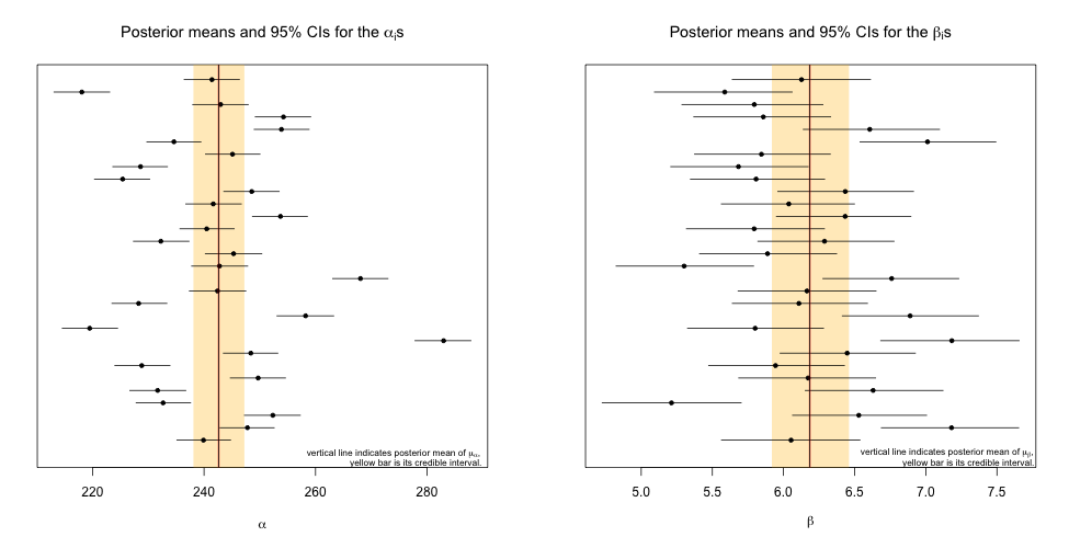
Question 1.3 Summarize your posterior inference about the 62 location parameters graphically.

Solution 1.3 To summarize inference about the \(\alpha\)s, we plot all 30 in addition to their respective 95% credible intervals. Within the same plot we include the posterior mean of \(\mu_\alpha\), the parameter that governs the center of the distribution that the \(\alpha\)s come from. A similar plot is generated for the \(\beta\)s.

Question 1.4 Graphically assess the sensitivity of \(\sigma_\alpha^2\) and \(\sigma_\beta^2\) to their respective priors.

Solution 1.4 For the posterior inference above, the priors for both \(\sigma_\alpha^2\) and \(\sigma_\beta^2\) were \(IG(a,b) = IG(5,5) \). To assess sensitivity, we'll generate Markov chains for other values of \(a\) and \(b\) and qualitatively evaluate how the posterior is affected.

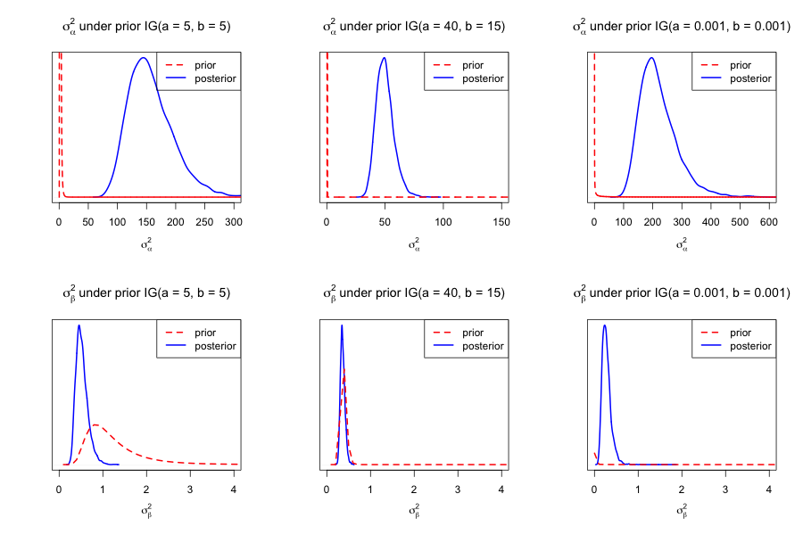
Posterior inference for \(\sigma^2_\alpha\) appears to be very sensitive to hyperparameter selection. Inference for \(\sigma^2_\beta\) displays some sensitivity, but not as much.

Question 1.5 For a noninformative prior, Prof. Andrew Gelman suggests using a truncated Uniform prior on the square root of the variance components.

Update the full conditionals and re-implement the Gibbs sampler.

Solution 1.5 The updated priors are now \(\sigma_\alpha \sim \text{Uniform}(0, A) \) and \(\sigma_\beta \sim \text{Uniform}(0, A) \) for some finite but sufficiently large \(A\). In other words, \(A\) is large enough such that \(\sigma_\alpha^2, \sigma_\beta^2 < A^2\), we never generate a variance value larger than \(A^2\).

In updating the full conditionals, only those for \(\sigma_\alpha^2\) and \(\sigma_\beta^2\) are affected:

• \( \begin{aligned} \pi(\sigma^2_\alpha \, | \, \text{other parameters, data}) \sim \; & % IG\left( \frac{n-1}{2}, \frac{1}{2} \sum_{i=1}^n ( \alpha_i-\mu_\alpha )^2 \right) \end{aligned} \)

  sa.update2 <- function(a, ma) {
      nua <- sum( (a - ma)^2 )
      return( 1 / rgamma(1, (n-1)/2, nua/2) )
  }
  

• \( \begin{aligned} \pi(\sigma^2_\beta \, | \, \text{other parameters, data}) \sim \; & % IG\left( \frac{n-1}{2}, \frac{1}{2} \sum_{i=1}^n ( \beta_i-\mu_\beta )^2 \right) \end{aligned} \)

  sb.update2 <- function(b, mb) {
      nub <- sum( (b - mb)^2 )
      return( 1 / rgamma(1, (n-1)/2, nub/2) )
  }
  

---